FSMfan
FSMfan computes confirmatory lrt of a suggested transformation
Description
Examples
 FSMfan with all default options.
FSMfan with all default options.First example with Mussels data.
load('mussels.mat');
Y=mussels{:,:};
warning('off','optim:fminunc:SwitchingMethod');
[out]=FSMfan(Y,[0.5 0 0.5 0 0]);
FSMfan with optional arguments.
FSMfan with optional arguments.Example with Mussels data.
load('mussels.mat');
Y=mussels{:,:};
% FS based on with H_0:\lambda=[1 0.5 1 0 1/3]
plotslrt=struct;
plotslrt.ylim=[-6.2 6.2];
warning('off','optim:fminunc:SwitchingMethod');
[out]=FSMfan(Y,[0.5 0 0.5 0 0],'laAround',[-1 -0.5 0 1/3 0.5 1],'init',58,'plotslrt',plotslrt);
% Compare this plot with Figure 4.24 p. 182 of ARC (2004)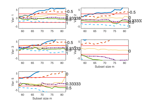
Related Examples
EmiliaRomagna data (demographic variables).
load('emilia2001')
Y=emilia2001{:,:};
% Replace zeros with min values for variables specified in sel
sel=[6 10 12 13 19 21];
for i=sel
Y(Y(:,i)==0,i)=min(Y(Y(:,i)>0,i));
end
% Extract demographic variables
Y1=Y(:,[1 2 3 4 5 10 11 12 13]);
colnames={'1' '2' '3' '4' '5' '10' '11' '12' '13'};
plotslrt=struct;
plotslrt.ylim=[-8.2 8.2];
la0=[0 0.25 0 0.5 0.5 0 0 0.5 0.25];
ColToComp=[1 3 5 9];
warning('off','optim:fminunc:SwitchingMethod');
[out]=FSMfan(Y1,la0,'ColToComp',ColToComp,'plotslrt',plotslrt,'colnames',colnames);
% Compare the plot Figure 4.35 p. 192 of ARC (2004)
Emilia Romagna data (modified wealth variables), example 1.
load('emilia2001')
Y=emilia2001{:,:};
% Replace zeros with min values for variables specified in sel
sel=[6 10 12 13 19 21];
for i=sel
Y(Y(:,i)==0,i)=min(Y(Y(:,i)>0,i));
end
% Modify wealth variables
Y(:,16)=100-Y(:,16);
Y(:,23)=100-Y(:,23);
% Extract wealth variables
Y1=Y(:,[14:23]);
colnames={'14' '15' '16' '17' '18' '19' '20' '21' '22' '23'};
plotslrt=struct;
plotslrt.ylim=[-8.2 8.2];
la0=[0 1 0.25 1 1 0.5 -0.5 0.25 0.25 -1];
ColToComp=[1 7];
warning('off','optim:fminunc:SwitchingMethod');
[out]=FSMfan(Y1,la0,'ColToComp',ColToComp,'plotslrt',plotslrt,'colnames',colnames);
% Compare the plot with the two upper panels of Figure 4.38 p. 188 of ARC (2004)
Emilia Romagna data (modified wealth variables), example 2.
load('emilia2001')
Y=emilia2001{:,:};
% Replace zeros with min values for variables specified in sel
sel=[6 10 12 13 19 21];
for i=sel
Y(Y(:,i)==0,i)=min(Y(Y(:,i)>0,i));
end
% Modify wealth variables
Y(:,16)=100-Y(:,16);
Y(:,23)=100-Y(:,23);
% Extract wealth variables
Y1=Y(:,[14:23]);
colnames={'14' '15' '16' '17' '18' '19' '20' '21' '22' '23'};
plotslrt=struct;
plotslrt.ylim=[-7 7];
la0=[0 1 0.25 1 1 0.5 -0.5 0.25 0.25 -1];
ColToComp=[3 9];
laAround=[0 0.25 1/3 0.5];
warning('off','optim:fminunc:SwitchingMethod');
[out]=FSMfan(Y1,la0,'laAround',laAround,'ColToComp',ColToComp,'plotslrt',plotslrt,'colnames',colnames);
% Compare the plot with the two bottom panels of Figure 4.39 p. 195 of ARC (2004)
Emilia Romagna data with Yeo and Johnson parametric family.
load('emilia2001')
Y=emilia2001{:,:};
% Modify wealth variables
Y(:,16)=100-Y(:,16);
Y(:,23)=100-Y(:,23);
% Extract wealth variables
Y1=Y(:,[14:23]);
colnames={'14' '15' '16' '17' '18' '19' '20' '21' '22' '23'};
plotslrt=struct;
plotslrt.ylim=[-7 7];
la0=[0 1 0.25 1 1 0.5 -0.5 0.25 0.25 -1];
ColToComp=[3 9];
laAround=[0 0.25 1/3 0.5];
warning('off','optim:fminunc:SwitchingMethod');
[out]=FSMfan(Y1,la0,'laAround',laAround,'ColToComp',ColToComp,'plotslrt',plotslrt,'colnames',colnames,'family','YJ');
Emilia Romagna data (modified work variables), example 1.
load('emilia2001')
Y=emilia2001{:,:};
% Replace zeros with min values for variables specified in sel
sel=[6 10 12 13 19 21 25 26];
for i=sel
Y(Y(:,i)==0,i)=min(Y(Y(:,i)>0,i));
end
% Extract work variables
Y1=Y(:,[6:9 24:28]);
colnames={'y6' 'y7' 'y8' 'y9' 'y24' 'y25' 'y26' 'y27' 'y28'};
la0=[0.25,0,2,-1,0,1.5,0.5,1,1];
plotslrt=struct;
plotslrt.ylim=[-8.2 8.2];
ColToComp=[1:4];
laAround=[-1 -0.5 0 0.25 0.5 1 2];
warning('off','optim:fminunc:SwitchingMethod');
[out]=FSMfan(Y1,la0,'ColToComp',ColToComp,'laAround',laAround,'plotslrt',plotslrt,'colnames',colnames);
% Compare the plot with Figure 4.43 p. 198 of ARC (2004)
Emilia Romagna data (modified work variables), example 2.
load('emilia2001')
Y=emilia2001{:,:};
% Replace zeros with min values for variables specified in sel
sel=[6 10 12 13 19 21];
for i=sel
Y(Y(:,i)==0,i)=min(Y(Y(:,i)>0,i));
end
% Modify variables 25 and 26
Y(:,25)=100-Y(:,25);
Y(:,26)=100-Y(:,26);
% Extract work variables
Y1=Y(:,[6:9 24:28]);
colnames={'y6' 'y7' 'y8' 'y9' 'y24' 'y25' 'y26' 'y27' 'y28'};
la0=[0.25,0,2,-1,0,0,1.5,1,1];
plotslrt=struct;
plotslrt.ylim=[-8.2 8.2];
ColToComp=[6 7];
laAround=[-1 -0.5 0 0.25 0.5 1 1.5 2];
warning('off','optim:fminunc:SwitchingMethod');
[out]=FSMfan(Y1,la0,'ColToComp',ColToComp,'laAround',laAround,'plotslrt',plotslrt,'colnames',colnames);
% Compare the plot with Figure 4.44 p. 199 of ARC (2004)
Emilia Romagna data (all variables).
load('emilia2001')
Y=emilia2001{:,:};
% Replace zeros with min values for variables specified in sel
sel=[6 10 12 13 19 21];
for i=sel
Y(Y(:,i)==0,i)=min(Y(Y(:,i)>0,i));
end
% Modify variables y16 y23 y25 y26
sel=[16 23 25 26];
Y(:,sel)=100-Y(:,sel);
colnames={'y6' 'y7' 'y8' 'y9' 'y24' 'y25' 'y26' 'y27' 'y28'};
la0demo=[0,0.25,0,0.5,0.5,0,0,0.5,0.25];
la0weal=[0,1,0.25,1,1,0.5,-0.5,0.25,0.25,-1];
la0work=[0.25,0,2,-1,0,0,1,1,1];
la0C1=[la0demo(1:5) la0work(1:4) la0demo(6:9) la0weal la0work(5:9)];
plotslrt=struct;
plotslrt.ylim=[-8.2 8.2];
ColToComp=[8 9 14 25];
laAround=[-1 -0.5 0 0.25 0.5 1 1.5 2];
warning('off','optim:fminunc:SwitchingMethod');
[out]=FSMfan(Y,la0C1,'ColToComp',ColToComp,'laAround',laAround,'plotslrt',plotslrt,'init',100);
% Compare the plot with Figure 4.45 p. 199 of ARC (2004)
Emilia Romagna data (all variables) with Yeo and Johnson parametric
family.
load('emilia2001')
Y=emilia2001{:,:};
% Replace zeros with min values for variables specified in sel
sel=[6 10 12 13 19 21];
for i=sel
Y(Y(:,i)==0,i)=min(Y(Y(:,i)>0,i));
end
% Modify variables y16 y23 y25 y26
sel=[16 23 25 26];
Y(:,sel)=100-Y(:,sel);
colnames={'y6' 'y7' 'y8' 'y9' 'y24' 'y25' 'y26' 'y27' 'y28'};
la0demo=[0,0.25,0,0.5,0.5,0,0,0.5,0.25];
la0weal=[0,1,0.25,1,1,0.5,-0.5,0.25,0.25,-1];
la0work=[0.25,0,2,-1,0,0,1,1,1];
la0C1=[la0demo(1:5) la0work(1:4) la0demo(6:9) la0weal la0work(5:9)];
plotslrt=struct;
plotslrt.ylim=[-8.2 8.2];
ColToComp=[8 9 14 25];
laAround=[-1 -0.5 0 0.25 0.5 1 1.5 2];
warning('off','optim:fminunc:SwitchingMethod');
[out]=FSMfan(Y,la0C1,'ColToComp',ColToComp,'laAround',laAround,'plotslrt',plotslrt,'init',100,'family','YJ');
Input Arguments
Y — Input data.
Matrix.
n x v data matrix; n observations and v variables. Rows of Y represent observations, and columns represent variables.
Missing values (NaN's) and infinite values (Inf's) are allowed, since observations (rows) with missing or infinite values will automatically be excluded from the computations.
Data Types: single|double
la0 — Transformation parameters.
Vector.
Vector of length v=size(Y,2) specifying a reasonable set of transformations for the columns of the multivariate data set.
Data Types: single | double
Name-Value Pair Arguments
Specify optional comma-separated pairs of Name,Value arguments.
Name is the argument name and Value
is the corresponding value. Name must appear
inside single quotes (' ').
You can specify several name and value pair arguments in any order as
Name1,Value1,...,NameN,ValueN.
 'family','YJ'
, 'rf',0.99
, 'init',50
, 'ColToComp',[1 3]
, 'laAround',[1 0]
,'optmin.Display','off'
, 'speed',0
, 'colnames',{'1' '2' '3' '4' '5' '10' '11' '12' '13'}
, 'signlr',0
,'plotslrt',1
, 'msg',0
family
—string which identifies the family of transformations which
must be used.character.
Possible values are 'BoxCox' (default) or 'YJ'.
The Box-Cox family of power transformations equals $(y^{\lambda}-1)/\lambda$ for $\lambda \neq 0$, and $log(y)$ if $\lambda = 0$.
The Yeo-Johnson (YJ) transformation is the Box-Cox transformation of y+1 for nonnegative values, and of |y|+1 with parameter $2-\lambda$ for y negative.
The basic power transformation returns $y^{\lambda}$ if $\lambda \neq 0$ and $log(\lambda)$ otherwise.
Remark. BoxCox and the basic power family can be used just if input y is positive. YeoJohnson family of transformations does not have this limitation.
Example: 'family','YJ'
Data Types: char
rf
—confidence level for bivariate ellipses.scalar.
Default is 0.9.
Example: 'rf',0.99
Data Types: double
init
—Point where to start monitoring required diagnostics.scalar.
Note that if bsb is supplied init>=length(bsb). If init is not specified it will be set equal to floor(n*0.6).
Example: 'init',50
Data Types: double
ColToComp
—variables for which likelihood ratio tests have to be
produced.vector.
It is a k x 1 integer vector. For example, if ColToComp = [2 4], the signed likelihood ratio tests are produced for the second and the fourth column of matrix Y.
If col.to.compare = '' then all variables (columns of matrix Y) are considered.
Example: 'ColToComp',[1 3]
Data Types: double
laAround
—It specifies for which values
of lambda to compute the likelihood ratio test.scalar.
It is a r x 1 vector. If this argument is omitted, the function produces for each variable specified in ColToComp the likelihood ratio tests associated to the five most common values of lambda [-1, -0.5, 0, 0.5, 1].
Example: 'laAround',[1 0]
Data Types: double
optmin
—It contains the options dealing with the
maximization algorithm.structure.
Use optimset to set these options.
Notice that the maximization algorithm which is used is fminunc if the optimization toolbox is present else is fminsearch.
Example: 'optmin.Display','off'
Data Types: double
speed
—It indicates the initial value of
the maximization procedure.scalar.
If speed=1 (default) the initial value at step m of the maximization procedure (fminunc or fminsearch) is the final value at step m-1 else it is la0.
Example: 'speed',0
Data Types: double
colnames
—the names of the variables of the dataset.cell array of strings.
Cell array of strings of length v containing the names of the variables of the dataset. If colnames is empty then the sequence 1:v is created to label the variables.
Example: 'colnames',{'1' '2' '3' '4' '5' '10' '11' '12' '13'}
Data Types: Cell array of strings.
signlr
—plots of signed square root
likelihood ratios.scalar.
If signlr = 1 (default) plots of signed square root likelihood ratios are produced, else likelihood ratios are produced.
Example: 'signlr',0
Data Types: double
plotslrt
—It specifies whether it is necessary to
plot the (signed square root) likelihood ratio test.scalar | structure.
If plotslrt is a scalar, the plot of the monitoring of likelihood ratio test is produced on the screen with all default options.
If plotslrt is a strucure, it may contain the following fields:
| Value | Description |
|---|---|
xlim |
minimum and maximum on the x axis; |
ylim |
minimum and maximum on the y axis; |
LineWidth |
Line width of the trajectory of lrt of transformation parameters; |
conflev |
vector which defines the confidence levels of the horizontal line for the likelihood ratio test (default is conflev=[0.95 0.99]); |
LineWidthEnv |
Line width of the horizontal lines; |
Tag |
tag of the plot (default is pl_lrt). |
Example: 'plotslrt',1
Data Types: double
msg
—Message on the screen.scalar.
It controls whether to display or not messages about great interchange on the screen. If msg==1 (default) messages are displyed on the screen else no message is displayed on the screen.
Example: 'msg',0
Data Types: double
Output Arguments
out — description
Structure
Structure which contains the following fields
| Value | Description |
|---|---|
LRT |
Cell of length ColtoComp. Each element of the cell contains the a matrix of size n-init+1 x length(laAround)+1 which contains the monitoring of (signed square root) likelihood ratio for testing H0:\lambda_j=la0_j when all the other variables are transformed as specified in vector la0. More precisely each matrix of size n-init+1 x length(laAround)+1 presents the following structure: 1st col = fwd search index (from init to n); 2nd col = value of the (signed sqrt) likelihood ratio for testing laj=laAround(1); ... length(laAround)+1 col = value of the (signed sqrt) likelihood ratio for testing laj=laAround(end). |
Exflag |
Cell of length ColtoComp. Each element of the cell contains the a matrix of size n-init+1 x length(laAround)+1 which contains the monitoring of the integer identifying the reason why the maximization algorithm terminated. See help page fminunc of the optimization toolbox for the list of values of exitflag and the corresponding reasons the algorithm terminated. More precisely each matrix of size n-init+1 x length(laAround)+1 presents the following structure: 1st col = fwd search index (from init to n); 2nd col = integer identifying the reason the algorithm terminated when testing laj=laAround(1); ... length(laAround)+1 col = integer identifying the reason the algorithm terminated when testing laj=laAround(end). |
Un |
Cell of length ColtoComp. Each element of the cell contains the a (sub)cell of size length(laAround). Each element of the (sub)cell contains a n-init+1 x 11 which informs the order of entry of the units For example Unj=Un{i}{j} refers to ColtoComp(i) and laAround(j) Unj is a (n-init) x 11 matrix which contains the unit(s) included in the subset at each step of the fwd search. REMARK: in every step the new subset is compared with the old subset. Un contains the unit(s) present in the new subset but not in the old one Unj(1,2) for example contains the unit included in step init+1 Unj(end,2) contains the units included in the final step of the search |
class |
'FSMfan'. |
References
Atkinson, A.C., Riani, M. and Cerioli, A. (2004), "Exploring multivariate data with the forward search", Springer Verlag, New York.