PDwei
PDwei computes weight function psi(u)/u for for minimum density power divergence estimator
Syntax
w=PDwei(u,alpha)example
Description
Examples
Related Examples
 Compare five different weight functions.
Compare five different weight functions.In each of them eff is 95 per cent.
% Initialize graphical parameters.
FontSize=14;
x=-6:0.01:6;
ylim1=-0.05;
ylim2=1.05;
xlim1=min(x);
xlim2=max(x);
LineWidth=2;
subplot(2,3,1)
ceff095HU=HUeff(0.95,1);
weiHU=HUwei(x,ceff095HU);
plot(x,weiHU,'LineWidth',LineWidth)
xlabel('$u$','Interpreter','Latex','FontSize',FontSize)
title('Huber','FontSize',FontSize)
ylim([ylim1 ylim2])
xlim([xlim1 xlim2])
subplot(2,3,2)
ceff095HA=HAeff(0.95,1);
weiHA=HAwei(x,ceff095HA);
plot(x,weiHA,'LineWidth',LineWidth)
xlabel('$u$','Interpreter','Latex','FontSize',FontSize)
title('Hampel','FontSize',FontSize)
ylim([ylim1 ylim2])
xlim([xlim1 xlim2])
subplot(2,3,3)
ceff095TB=TBeff(0.95,1);
weiTB=TBwei(x,ceff095TB);
plot(x,weiTB,'LineWidth',LineWidth)
xlabel('$u$','Interpreter','Latex','FontSize',FontSize)
title('Tukey biweight','FontSize',FontSize)
ylim([ylim1 ylim2])
xlim([xlim1 xlim2])
subplot(2,3,4)
ceff095HYP=HYPeff(0.95,1);
ktuning=4.5;
weiHYP=HYPwei(x,[ceff095HYP,ktuning]);
plot(x,weiHYP,'LineWidth',LineWidth)
xlabel('$u$','Interpreter','Latex','FontSize',FontSize)
title('Hyperbolic','FontSize',FontSize)
ylim([ylim1 ylim2])
xlim([xlim1 xlim2])
subplot(2,3,5)
ceff095PD=PDeff(0.95);
weiPD=PDwei(x,ceff095PD);
weiPD=weiPD/max(weiPD);
plot(x,weiPD,'LineWidth',LineWidth)
xlabel('$u$','Interpreter','Latex','FontSize',FontSize)
title('Power divergence','FontSize',FontSize)
ylim([ylim1 ylim2])
xlim([xlim1 xlim2])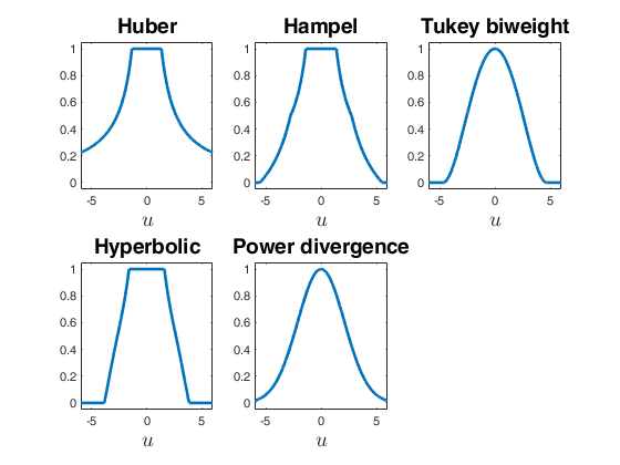
Input Arguments
Output Arguments
More About
References
Riani, M. Atkinson, A.C., Corbellini A. and Perrotta A. (2020), Robust Regression with Density Power Divergence: Theory, Comparisons and Data Analysis, Entropy, Vol. 22, 399.