Smulteda
Smulteda computes S estimators in multivariate analysis for a series of values of bdp
Syntax
Description
Examples
Smulteda with all default options.
n=200;
v=3;
randn('state', 123456);
Y=randn(n,v);
% Contaminated data
Ycont=Y;
Ycont(1:5,:)=Ycont(1:5,:)+3;
[out]=Smulteda(Ycont);
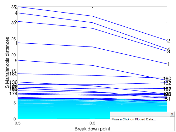
 Smulteda with optional arguments.
Smulteda with optional arguments.
n=200;
v=3;
randn('state', 123456);
Y=randn(n,v);
% Contaminated data
Ycont=Y;
Ycont(1:5,:)=Ycont(1:5,:)+3;
[out]=Smulteda(Ycont,'bdp',[0.5 0.3 0.1],'plots',1);
Total estimated time to complete S estimator: 1.12 seconds Total estimated time to complete S estimator: 0.42 seconds Total estimated time to complete S estimator: 0.54 seconds
Smulteda with extracted subsamples.
n=200;
v=3;
randn('state', 123456);
Y=randn(n,v);
% Contaminated data
Ycont=Y;
Ycont(1:5,:)=Ycont(1:5,:)+3;
[out,C]=Smulteda(Ycont,'plots',1);
Input Arguments
Y — Input data.
Matrix.
n x v data matrix; n observations and v variables. Rows of Y represent observations, and columns represent variables.
Missing values (NaN's) and infinite values (Inf's) are allowed, since observations (rows) with missing or infinite values will automatically be excluded from the computations.
Data Types: single|double
Name-Value Pair Arguments
Specify optional comma-separated pairs of Name,Value arguments.
Name is the argument name and Value
is the corresponding value. Name must appear
inside single quotes (' ').
You can specify several name and value pair arguments in any order as
Name1,Value1,...,NameN,ValueN.
 'bdp',[0.5 0.4 0.3 0.2 0.1]
, 'nsamp',1000
, 'refsteps',0
, 'reftol',1e-8
, 'refstepsbestr',10
, 'reftolbestr',1e-10
, 'minsctol',1e-7
, 'bestr',10
, 'conflev',0.99
, 'nocheck',1
, 'plots',0
, 'msg',0
, 'ysave',1
bdp
—breakdown point.scalar | vector.
It measures the fraction of outliers the algorithm should resist. In this case any value greater than 0 but smaller or equal than 0.5 will do fine.
The default value of bdp is a sequence from 0.5 to 0.01 with step 0.01
Example: 'bdp',[0.5 0.4 0.3 0.2 0.1]
Data Types: double
nsamp
—Number of subsamples which will be extracted to find the
robust estimator.scalar.
If nsamp=0 all subsets will be extracted.
They will be (n choose p).
If the number of all possible subset is <1000 the default is to extract all subsets otherwise just 1000.
Example: 'nsamp',1000
Data Types: single | double
refsteps
—Number of refining iterations.scalar.
Number of refining iterationsin each subsample (default = 3).
refsteps = 0 means "raw-subsampling" without iterations.
Example: 'refsteps',0
Data Types: single | double
reftol
—scalar.default value of tolerance for the refining steps.
The default value is 1e-6;
Example: 'reftol',1e-8
Data Types: single | double
refstepsbestr
—number of refining iterations for each best subset.scalar.
Scalar defining number of refining iterations for each best subset (default = 50).
Example: 'refstepsbestr',10
Data Types: single | double
reftolbestr
—Tolerance for the refining steps.scalar.
Tolerance for the refining steps for each of the best subsets The default value is 1e-8;
Example: 'reftolbestr',1e-10
Data Types: single | double
minsctol
—tolerance for the iterative
procedure for finding the minimum value of the scale.scalar.
Value of tolerance for the iterative procedure for finding the minimum value of the scale for each subset and each of the best subsets (It is used by subroutine minscale.m) The default value is 1e-7;
Example: 'minsctol',1e-7
Data Types: single | double
bestr
—number of "best betas" to remember.scalar.
Scalar defining number of "best betas" to remember from the subsamples. These will be later iterated until convergence (default=5)
Example: 'bestr',10
Data Types: single | double
conflev
—Confidence level which is
used to declare units as outliers.scalar.
Usually conflev=0.95, 0.975 0.99 (individual alpha) or 1-0.05/n, 1-0.025/n, 1-0.01/n (simultaneous alpha).
Default value is 0.975
Example: 'conflev',0.99
Data Types: double
nocheck
—Check input arguments.scalar.
If nocheck is equal to 1 no check is performed on matrix Y. As default nocheck=0.
Example: 'nocheck',1
Data Types: double
plots
—Plot on the screen.scalar | structure.
If plots is a structure or scalar equal to 1, generates:
(1) a plot of Mahalanobis distances against index number. The confidence level used to draw the confidence bands for the MD is given by the input option conflev. If conflev is not specified a nominal 0.975 confidence interval will be used.
(2) a scatter plot matrix with the outliers highlighted.
If plots is a structure it may contain the following fields
| Value | Description |
|---|---|
labeladd |
if this option is '1', the outliers in the spm are labelled with their unit row index. The default value is labeladd='', i.e. no label is added. |
nameY |
cell array of strings containing the labels of the variables. As default value, the labels which are added are Y1, ...Yv. |
Example: 'plots',0
Data Types: single | double
msg
—Level of output to display.scalar.
If msg==1 (default) messages are displayed on the screen about estimated time to compute the final estimator else no message is displayed on the screen
Example: 'msg',0
Data Types: single | double
ysave
—save input matrix Y.scalar.
Scalar that is set to 1 to request that the data matrix Y is saved into the output structure out. This feature is meant at simplifying the use of function malindexplot.
Default is 0, i.e. no saving is done.
Example: 'ysave',1
Data Types: double
Output Arguments
out — description
Structure
A structure containing the following fields
| Value | Description |
|---|---|
Loc |
length(bdp)-by-v matrix containing S estimate of location for each value of bdp |
Shape |
v-by-v-by-length(bdp) 3D array containing robust estimate of the shape for each value of bdp. Remark det|shape|=1 |
Scale |
length(bdp) vector. Robust estimate of the scale for each value of bdp |
cov |
v-by-v-by-length(bdp) 3D array containing robust estimate of Note that out.scale(i)^2 * out.shape(:,:,i) = robust estimate of covariance matrix |
BS |
(v+1)-by-length(bdp) matrix containing the units forming best subset for each value of bdp |
MAL |
n-by-length(bdp) matrix containing the estimates of the robust Mahalanobis distances (in squared units) for each value of bdp |
Outliers |
n-by-length(bdp) matrix containing true for the outliers. Boolean matrix containing the list of the units declared as outliers for each value of bdp using confidence level specified in input scalar conflev |
Weights |
n x length(eff) matrix containing the weights for each value of eff |
conflev |
Confidence level that was used to declare outliers |
singsub |
Number of subsets without full rank. Notice that out.singsub > 0.1*(number of subsamples) produces a warning |
bdp |
vector which contains the values of bdp which have been used |
Y |
Data matrix Y. The field is present if option ysave is set to 1. |
class |
'Smulteda' |
References
Maronna, R.A., Martin D. and Yohai V.J. (2006), "Robust Statistics, Theory and Methods", Wiley, New York.