add2yX
add2yX adds objects (personalized clickable multilegends and text labels) to the yXplot
Description
Examples
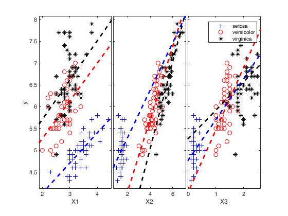
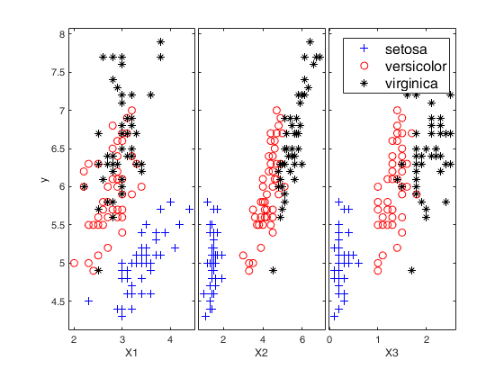
 Compare gplotmatrix and addyX with yXplot for IRIS data.
 Compare gplotmatrix and addyX with yXplot for IRIS data.
load fisheriris;
% Create scatter plot matrix with specific legends
% plot Sepal length (y) againt the other variables
y=meas(:,1);
X=meas(:,2:4);
[H,AX,BigAx]=gplotmatrix(X,y,species,[],[],[],'on');
% The legends are not clickable
add2yX(H,AX,BigAx)
% Now the legends become clickable
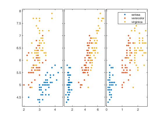
% It is easier to call directly function yXplot
[H,AX,BigAx]=yXplot(meas(:,1),meas(:,2:4),species);
Related Examples
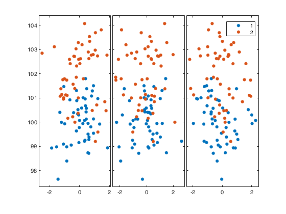
 Example of use of option 'labeladd' combined with 'RowNamesLabels'.
 Example of use of option 'labeladd' combined with 'RowNamesLabels'.
close all;
n=8;
y = randn(n,1);
X = randn(n,3);
group = ones(n,1);
group(1:5) = 2;
[H,AX,BigAx] = yXplot(y,X,group);
% Create cell containing the name of the rows.
label={'ddf1' 'ddf2' 'ddf3' 'ddf4' 'ddf5' 'ddf6' 'ddf7' 'ddf8'};
% Labels are added to the units which belong to group 2 (that is to the
% first 5 units). The labels are taken from cell label
add2yX(H,AX,BigAx,'labeladd','1','RowNamesLabels',label);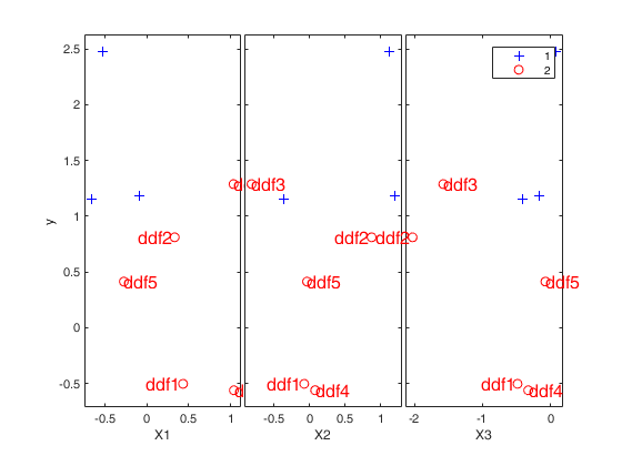
Input Arguments
H — handles to the lines on the graphs.
2D or 3D array.
H is an array of handles to the lines on the graphs. The array's third dimension corresponds to groups in the grouping variable. For more details see the output arguments of gplotmatrix.
Data Types: single| double
AX — handles to the axes of the individual plots.
Matrix.
AX is a matrix of handles to the axes of the individual plots.
For more details see the output arguments of gplotmatrix.
Data Types: single| double
BigAx — handle to big (invisible) axes framing the
entire plot matrix.
Scalar.
For more details see the output arguments of gplotmatrix.
Data Types: single| double
Name-Value Pair Arguments
Specify optional comma-separated pairs of Name,Value arguments.
Name is the argument name and Value
is the corresponding value. Name must appear
inside single quotes (' ').
You can specify several name and value pair arguments in any order as
Name1,Value1,...,NameN,ValueN.
 'bivarfit','1'
, 'multivarfit','1'
, 'labeladd','1'
, 'intercept',1
, 'userleg','1'
, 'RowNamesLabels',{'a' 'bb' 'cc' 'mmm'}
bivarfit
—Add a line fit.char.
'0' fit a line to each group;
'1' fit 1 line to all data, regardless the groups;
'2' fit a line on all data and a line to relevant data;
'' the default, nothing is added.
Example: 'bivarfit','1'
Data Types: char
multivarfit
—Add a multivariate fit.char.
'1' one multivariate fit on all units '2' one multivariate fit on all units and one on relevant data '' the default, nothing is added
Example: 'multivarfit','1'
Data Types: char
labeladd
—Add labels.char.
'1' add labels to relevant units '' the default, nothing is added
Example: 'labeladd','1'
Data Types: char
intercept
—Indicator for constant term.scalar.
intercept = 1 (default) assumes the intercept for the bivarfit and multivarfit. When intercept = 0, the intercept is not used for the fits.
Example: 'intercept',1
Data Types: double
userleg
—user legend.char.
It is used to control the legend of the plot.
- Default is ''. In this case, existing legends are left as they are and simply made clickable; however, if there is no legend, a default one is created using the syntax 'Group 1', 'Group 2', etc.
- If it is set to '1', the legends are updated depending on the context of use and are made clickable. The context is determined by the occurence of specific words in the Tag of the current figure. The strings/contexts currently addressed are: 'outlier' (for 'Outliers' and 'Normal units'), 'brush' (for 'Brushed units 1', 'Brushed units 2', etc.), 'group' (for 'Group 1', 'Group 2', etc.), '' i.e. the Tag of the figure is not defined;
in this case the legend takes the values in the DisplayName property of the scatter matrix. This is determined by the 'group' option of the spmplot or gplotmatrix functions.
- If it is a cell of strings, e.g. {'FIAT' ; 'BMW' ; 'VOLVO'}, then such strings are used for the legend.
Example: 'userleg','1'
Data Types: char
RowNamesLabels
—cell of length n, where n is the number of points in
each scatter, containing the labels of the units.if this field is empty the sequence 1:n will be used to label the units.
Example: 'RowNamesLabels',{'a' 'bb' 'cc' 'mmm'}
Data Types: cell
Output Arguments
More About
Additional Details
add2yX essentially used within FSDA function yXplot. However its logic can be also demonstrated with MATLAB function gplotmatrix, as in the examples below.
As default add2yX makes legends in the existing yX plot matrix clickable or creates a clickable multilegend if the legend does not exist.
Note that the function extracts the data from the graphical objects in the plot. At the current stage the objects that can be added to yXplot using add2yX are: - a bivariate fit on each panel of yXplot (see olsline.m);
- a multivariate fit that is shown on each panel of yXplt;
- the labels of relevant observations, e.g. outliers or brushed groups.
References
Tufte E.R. (1983), "The visual display of quantitative information", Graphics Press, Cheshire.
