balloonplot
balloonplot creates a balloon plot of a contingency table
Syntax
Description
A balloonplot is an alternative to bar plot for visualizing a large categorical data. It draws a graphical matrix of a contingency table, where each cell contains a dot whose size reflects the relative magnitude of the corresponding component. ballonplot is a bubble chart for contingency tables.
balloonplot with array input.h
=balloonplot(N,
Name, Value)
Examples
 balloonplot with table input.
balloonplot with table input.Load the Housetasks data (a contingency table containing the frequency of execution of 13 house tasks in the couple).
N=[156	14	2	4;
124	20	5	4;
77	11	7	13;
82	36	15	7;
53	11	1	57;
32	24	4	53;
33	23	9	55;
12	46	23	15;
10	51	75	3;
13	13	21	66;
8	1	53	77;
0	3	160	2;
0	1	6	153];
rowslab={'Laundry' 'Main-meal' 'Dinner' 'Breakfast' 'Tidying' 'Dishes' ...
'Shopping' 'Official' 'Driving' 'Finances' 'Insurance'...
'Repairs' 'Holidays'};
colslab={'Wife'	'Alternating'	'Husband'	'Jointly'};
tableN=array2table(N,'VariableNames',colslab,'RowNames',rowslab);
% In this case a table is supplied
balloonplot(tableN);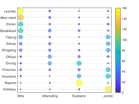
balloonplot with original data matrix as input.
balloonplot with original data matrix as input.
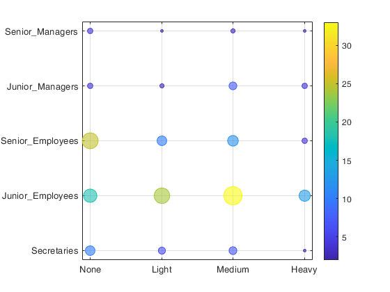
load smoke
[h,Ntable]=balloonplot(smoke,'datamatrix',true);
disp(Ntable)
                        None    Light    Medium    Heavy
                        ____    _____    ______    _____

    Senior_Managers       4       2         3        2
    Junior_Managers       4       3         7        4
    Senior_Employees     25      10        12        4
    Junior_Employees     18      24        33       13
    Secretaries          10       6         7        2
Related Examples
balloonplot with option contrib2Index as boolean.
balloonplot with option contrib2Index as boolean.Load the Housetasks data (a contingency table containing the frequency of execution of 13 house tasks in the couple).
% This ia a German sample in young, married, heterosexual couples in the late 1970s,
N=[156	14	2	4;
124	20	5	4;
77	11	7	13;
82	36	15	7;
53	11	1	57;
32	24	4	53;
33	23	9	55;
12	46	23	15;
10	51	75	3;
13	13	21	66;
8	1	53	77;
0	3	160	2;
0	1	6	153];
rowslab={'Laundry' 'Main-meal' 'Dinner' 'Breakfast' 'Tidying' 'Dishes' ...
'Shopping' 'Official' 'Driving' 'Finances' 'Insurance'...
'Repairs' 'Holidays'};
colslab={'Wife'	'Alternating'	'Husband'	'Jointly'};
% If the DimensionNames is set the xlabel and ylabel will be added
% automatically.
Ntable=array2table(N,'VariableNames',colslab,'RowNames',rowslab);
Ntable.Properties.DimensionNames=["Repartition in the couple" "13 housetasks"];
% Call to balloonplot with option 'contrib2Index' boolean equal to
% true. In this case the contributions to the Chi2 statistic
% are shown. The color is associated to the sign.
balloonplot(Ntable,'contrib2Index',true);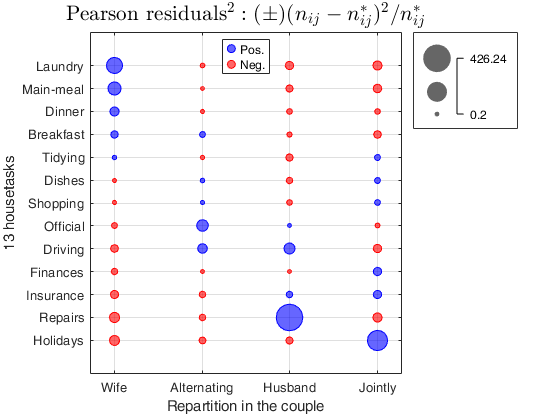
Example of ballonplot with option contrib2Index as a matrix.
Example of ballonplot with option contrib2Index as a matrix.
load SportHealth.mat
out=corrOrdinal(SportHealth);
balloonplot(SportHealth,'contrib2Index',out.Contrib2CminusD)
title(['Indice \gamma=' num2str(out.gam(1))])
Test of H_0: independence between rows and columns
The standard errors are computed under H_0
              Coeff        se       zscore    pval
             _______    ________    ______    ____

    gamma    0.59385    0.053088    11.186     0
    taua     0.33958     0.03852    8.8157     0
    taub     0.45635    0.040796    11.186     0
    tauc     0.45128    0.040343    11.186     0
    dyx       0.4525    0.040451    11.186     0

-----------------------------------------
Indexes and 95% confidence limits
The standard error are computed under H_1
              Value     StandardError    ConflimL    ConflimU
             _______    _____________    ________    ________

    gamma    0.59385       0.04837       0.49905     0.68866
    taua     0.33958      0.011291       0.31745     0.36171
    taub     0.45635      0.040331        0.3773      0.5354
    tauc     0.45128      0.040343       0.37221     0.53036
    dyx       0.4525      0.040106       0.37389     0.53111


ans =

  Figure (pl_balloonplot) with properties:

      Number: 4
        Name: ''
       Color: [0.9608 0.9608 0.9608]
    Position: [1 1 1536 744]
       Units: 'pixels'

  Use GET to show all properties
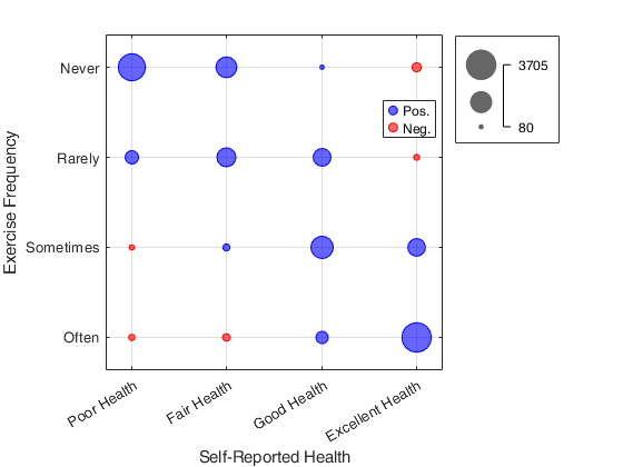
Example where contrib2Index is a table.
Example where contrib2Index is a table.
load SportHealth.mat
out=corrNominal(SportHealth);
out.Contrib2Hyxtable
% Contribution to Hyx index from each cell of the table
balloonplot(SportHealth,'contrib2Index', out.Contrib2Hyxtable)
title(['Contribution of each single cell to Hyx=' num2str(out.Hyx(1))])
Chi2 index
  104.4294

pvalue Chi2 index
   1.9934e-18

Phi index
    0.5871

Cramer's V
    0.3389

Test of H_0: independence between rows and columns
                   Coeff        se       zscore       pval
                  _______    ________    ______    __________

    CramerV       0.33895    0.040732    8.3214             0
    GKlambdayx    0.19307    0.044247    4.3634    1.2803e-05
    tauyx         0.11153    0.021133    5.2774    1.3104e-07
    Hyx           0.12654    0.022713    5.5711     2.531e-08

-----------------------------------------
Indexes and 95% confidence limits
                   Value     StandardError    ConflimL    ConflimU
                  _______    _____________    ________    ________

    CramerV       0.33895      0.040732        0.25911    0.39187
    GKlambdayx    0.19307      0.044247        0.10635    0.27979
    tauyx         0.11153      0.021133       0.070107    0.15295
    Hyx           0.12654      0.022713       0.082019    0.17105


ans =

  4×4 table

                 Poor Health    Fair Health    Good Health    Excellent Health
                 ___________    ___________    ___________    ________________

    Never          0.065383       0.030991      -0.020606        -0.016491
    Rarely        0.0011911        0.01432      0.0059075        -0.015609
    Sometimes     -0.012717      -0.013736        0.04043        0.0057804
    Often        -0.0086721        -0.0125     -0.0060879         0.068952


ans =

  Figure (pl_balloonplot) with properties:

      Number: 5
        Name: ''
       Color: [0.9608 0.9608 0.9608]
    Position: [1 1 1536 744]
       Units: 'pixels'

  Use GET to show all properties