CorAnaplot
CorAnaplot draws the Correspondence Analysis (CA) graphs with confidence ellipses.
Examples
 CorAnaplot with all the default options.
CorAnaplot with all the default options.Prepare the data.
N=[51 64 32 29 17 59 66 70;
53 90 78 75 22 115 117 86;
71 111 50 40 11 79 88 177;
1 7 5 5 4 9 8 5;
7 11 4 3 2 2 17 18;
7 13 12 11 11 18 19 17;
21 37 14 26 9 14 34 61;
12 35 19 6 7 21 30 28;
10 7 7 3 1 8 12 8;
4 7 7 6 2 7 6 13;
8 22 7 10 5 10 27 17;
25 45 38 38 13 48 59 52;
18 27 20 19 9 13 29 53;
35 61 29 14 12 30 63 58;
2 4 3 1 4 nan nan nan ;
2 8 2 5 2 nan nan nan;
1 5 4 6 3 nan nan nan;
3 3 1 3 4 nan nan nan];
% rowslab = cell containing row labels
rowslab={'money','future','unemployment','circumstances',...
'hard','economic','egoism','employment','finances',...
'war','housing','fear','health','work','comfort','disagreement',...
'world','to_live'};
% colslab = cell containing column labels
colslab={'unqualified','cep','bepc','high_school_diploma','university',...
'thirty','fifty','more_fifty'};
if verLessThan('matlab','8.2.0')==0
tableN=array2table(N,'VariableNames',colslab,'RowNames',rowslab);
% Extract just active rows
Nactive=tableN(1:14,1:5);
Nsupr=tableN(15:18,1:5);
Nsupc=tableN(1:14,6:8);
Sup=struct;
Sup.r=Nsupr;
Sup.c=Nsupc;
% Compute Correspondence analysis
else
Nactive=N(1:14,1:5);
Lr=rowslab(1:14);
Lc=colslab(1:5);
Sup=struct;
Sup.r=N(15:end,1:5);
Sup.Lr=rowslab(15:end);
Sup.c=N(1:14,6:8);
Sup.Lc=colslab(6:8);
end
% Compute correspondence analysis
out=CorAna(Nactive,'Sup',Sup,'plots',0,'dispresults',false);
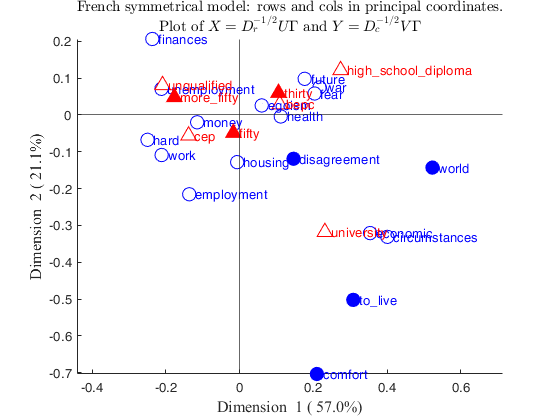
% Show the correspondence analysis plot.
% Rows and columns are shown in principal coordinates
CorAnaplot(out)
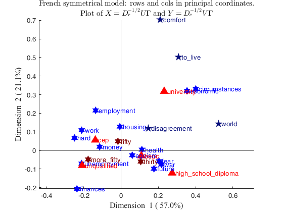
CorAnaplot with personalized symbols.
CorAnaplot with personalized symbols.
close all
% Prepare the data.
N=[51  64  32  29  17  59  66  70;
53  90  78  75  22  115  117  86;
71  111  50  40  11  79  88  177;
1  7  5  5  4  9  8  5;
7  11  4  3  2  2  17  18;
7  13  12  11  11  18  19  17;
21  37  14  26  9  14  34  61;
12  35  19  6  7  21  30  28;
10  7  7  3  1  8  12  8;
4  7  7  6  2  7  6  13;
8  22  7  10  5  10  27  17;
25  45  38  38  13  48  59  52;
18  27  20  19  9  13  29  53;
35  61  29  14  12  30  63  58;
2  4  3  1  4  nan  nan  nan    ;
2  8  2  5  2  nan  nan  nan;
1  5  4  6  3  nan  nan  nan;
3  3  1  3  4  nan  nan  nan];
% rowslab = cell containing row labels
rowslab={'money','future','unemployment','circumstances',...
'hard','economic','egoism','employment','finances',...
'war','housing','fear','health','work','comfort','disagreement',...
'world','to_live'};
% colslab = cell containing column labels
colslab={'unqualified','cep','bepc','high_school_diploma','university',...
'thirty','fifty','more_fifty'};
if verLessThan('matlab','8.2.0')==0
tableN=array2table(N,'VariableNames',colslab,'RowNames',rowslab);
% Extract just active rows
Nactive=tableN(1:14,1:5);
Nsupr=tableN(15:18,1:5);
Nsupc=tableN(1:14,6:8);
Sup=struct;
Sup.r=Nsupr;
Sup.c=Nsupc;
% Compute Correspondence analysis
else
Nactive=N(1:14,1:5);
Lr=rowslab(1:14);
Lc=colslab(1:5);
Sup=struct;
Sup.r=N(15:end,1:5);
Sup.Lr=rowslab(15:end);
Sup.c=N(1:14,6:8);
Sup.Lc=colslab(6:8);
end
% Six-pointed star (hesagram) for supplementary rows
SymbolRows='h';
% Five-pointed star (pentagram) for supplementary rows
SymbolRowsSup='p';
% Color for active rows
ColorRows='b';
% Color for supplementary rows (dark blue)
ColorRowsSup=[6 13 123]/255;
% Blue fill color for active rows
MarkerFaceColorRows='b';
% Right-pointing triangle for active columns
Symbolcols='^';
% Six-pointed star (hexagram) for supplementary columns
SymbolcolsSup='h';
% Color for active columns
ColorCols='r';
% Red fill color for active rows
MarkerFaceColorCols='r';
% Color for supplementary columns (dark red)
ColorColsSup=[128 0 0]/255;
plots=struct;
plots.SymbolRows=SymbolRows;
plots.SymbolRowsSup=SymbolRowsSup;
plots.ColorRows=ColorRows;
plots.ColorRowsSup=ColorRowsSup;
plots.MarkerFaceColorRows=MarkerFaceColorRows;
plots.SymbolCols=Symbolcols;
plots.SymbolColsSup=SymbolcolsSup;
plots.ColorCols=ColorCols;
plots.ColorColsSup=ColorColsSup;
plots.MarkerFaceColorCols=MarkerFaceColorCols;
% change the sign of the second dimension
changedimsign=[false true];
out=CorAna(Nactive,'Sup',Sup,'plots',0,'dispresults',false);
CorAnaplot(out,'plots',plots,'changedimsign',changedimsign)
Related Examples
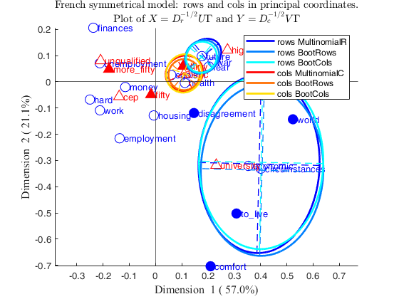
Correspondence analysis plot with selected ellipses.
Correspondence analysis plot with selected ellipses.
N=[51  64  32  29  17  59  66  70;
53  90  78  75  22  115  117  86;
71  111  50  40  11  79  88  177;
1  7  5  5  4  9  8  5;
7  11  4  3  2  2  17  18;
7  13  12  11  11  18  19  17;
21  37  14  26  9  14  34  61;
12  35  19  6  7  21  30  28;
10  7  7  3  1  8  12  8;
4  7  7  6  2  7  6  13;
8  22  7  10  5  10  27  17;
25  45  38  38  13  48  59  52;
18  27  20  19  9  13  29  53;
35  61  29  14  12  30  63  58;
2  4  3  1  4  nan  nan  nan    ;
2  8  2  5  2  nan  nan  nan;
1  5  4  6  3  nan  nan  nan;
3  3  1  3  4  nan  nan  nan];
% rowslab = cell containing row labels
rowslab={'money','future','unemployment','circumstances',...
'hard','economic','egoism','employment','finances',...
'war','housing','fear','health','work','comfort','disagreement',...
'world','to_live'};
% colslab = cell containing column labels
colslab={'unqualified','cep','bepc','high_school_diploma','university',...
'thirty','fifty','more_fifty'};
if verLessThan('matlab','8.2.0')==0
tableN=array2table(N,'VariableNames',colslab,'RowNames',rowslab);
% Extract just active rows
Nactive=tableN(1:14,1:5);
Nsupr=tableN(15:18,1:5);
Nsupc=tableN(1:14,6:8);
Sup=struct;
Sup.r=Nsupr;
Sup.c=Nsupc;
else
Nactive=N(1:14,1:5);
Lr=rowslab(1:14);
Lc=colslab(1:5);
Sup=struct;
Sup.r=N(15:end,1:5);
Sup.Lr=rowslab(15:end);
Sup.c=N(1:14,6:8);
Sup.Lc=colslab(6:8);
end
% Superimpose confidence ellipses for rows 2 and 4 and for column 3
confellipse=struct;
confellipse.selRows=[2 4];
% Ellipse for column 3 using an integer
confellipse.selCols=3;
% Ellipse for column 3 using a Boolean vector
confellipse.selCols=[ false false true false false];
% confellipse.selCols={'c3'};
% Use the 3 methods below in order to compute the confidence ellipses for
% the selected rows and columns of the input contingency table
confellipse.method={'multinomial' 'bootRows' 'bootCols'};
% Set number of simulations
confellipse.nsimul=500;
% Set confidence interval
confellipse.conflev=0.50;
out=CorAna(Nactive,'Sup',Sup,'plots',0,'dispresults',false);
% Draw correspondence analysis plot with requested confidence ellipses
CorAnaplot(out,'plots',1,'confellipse',confellipse)
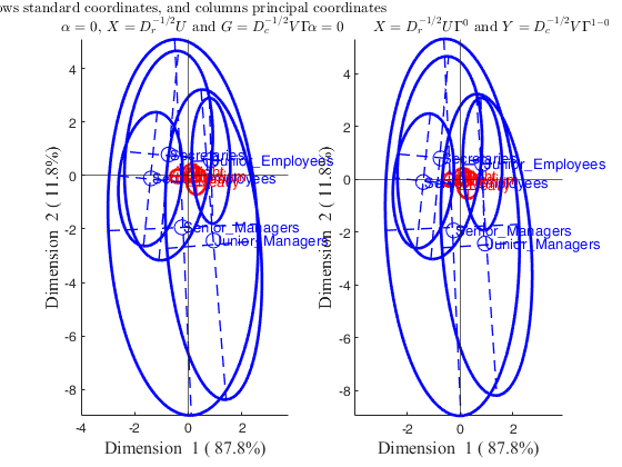
Correpondence analysis of the smoke data.
Correpondence analysis of the smoke data.In this example we compare the results which are obtained using option plots.alpha='colprincipal'; (which implicitly implies alpha=0) with those which come out imposing directly plots.alpha=0.
load smoke
[N,~,~,labels]=crosstab(smoke{:,1},smoke{:,2});
[I,J]=size(N);
labels_rows=labels(1:I,1);
labels_columns=labels(1:J,2);
out=CorAna(N,'Lr',labels_rows,'Lc',labels_columns,'plots',0,'dispresults',false);
plots=struct;
plots.alpha='rowgab';
plots.alpha='colgab';
plots.alpha='rowgreen';
plots.alpha='colgreen';
% Add confidence ellipses
confellipse=1;
plots.alpha='bothprincipal';
plots.alpha='rowprincipal';
plots.alpha='colprincipal';
h1=subplot(1,2,1);
CorAnaplot(out,'plots',plots,'confellipse',confellipse,'h',h1)
h2=subplot(1,2,2);
plots.alpha=0;
CorAnaplot(out,'plots',plots,'confellipse',confellipse,'h',h2);
Input Arguments
Output Arguments
References
Benzecri, J.-P. (1992), "Correspondence Analysis Handbook", New-York, Dekker.
Benzecri, J.-P. (1980), "L'analyse des donnees tome 2: l'analyse des correspondances", Paris, Bordas.
Greenacre, M.J. (1993), "Correspondence Analysis in Practice", London, Academic Press.
Gabriel, K.R. and Odoroff, C. (1990), Biplots in biomedical research, "Statistics in Medicine", Vol. 9, pp. 469-485.
Greenacre, M.J. (1993), Biplots in correspondence Analysis, "Journal of Applied Statistics", Vol. 20, pp. 251-269.
Riani, M, Atkinson A.C., Torti, F., Corbellini A. (2023), Robust Correspondence Analysis, "Journal of the Royal Statistical Society Series C: Applied Statistics", Vol. 71, pp. 1381–1401, https://doi.org/10.1111/rssc.12580
Urbano, L.-S., van de Velden, M. and Kiers, H.A.L. (2009), CAR: A MATLAB Package to Compute Correspondence Analysis with Rotations, "Journal of Statistical Software", Vol. 31.