mcdCorAna
mcdCorAna computes Minimum Covariance Determinant in correspondence analysis
Syntax
Description
Examples
 mcdCorAna with bdp=0.
 mcdCorAna with bdp=0.
N=[  69    46    41    13    22    18
29    52    45     3     5     3
19    55    47     2     3     1
50    22    19     8    10     7
25    38    33     2     4     3
30     2     1    45     8     2
35     6     5    32     5     2
28    12     7     7     5     4
26    12    11    11     4     3
21     6     4     3     3     2];
rowlab={'Teens' 'PicksYouUp' 'Energy' 'EnjoyLife' ...
'WhenTired' 'Kids' 'Fun' 'Refreshes' ...
'CheersYouUp' 'Relax'};
collab={'Coke' 'V' 'RedBull' 'Fanta' 'Pepsi' 'DietCoke'};
Ntable=array2table(N,'RowNames',rowlab,'VariableNames',collab);
RAW=mcdCorAna(Ntable,'bdp',0);
% Note that in this case RAW.md is equal to
% out.OverviewRows.Inertia./out.OverviewRows.Mass
% out = output from traditional correspondence analysis.
out=CorAna(Ntable,'dispresults',false,'plots',0);
d2=out.OverviewRows.Inertia./out.OverviewRows.Mass;
disp('Square distance of each row profile from the centroid')
disp([RAW.md d2])
The MCD estimates are equal to the classical estimates h=n=1036
Square distance of each row profile from the centroid
0.10 0.10
0.29 0.29
0.52 0.52
0.09 0.09
0.24 0.24
1.65 1.65
0.80 0.80
0.12 0.12
0.05 0.05
0.25 0.25
Example 1 of findEmpiricalEnvelope passed as struct.
load clothes.mat
findEmp=struct;
% Number of simulations to create the envelope
findEmp.nsimul=100;
% Simulate contingency tables with a Chi2 equal to the observed
findEmp.underH0=false;
% Set confidence level
conflev=0.95;
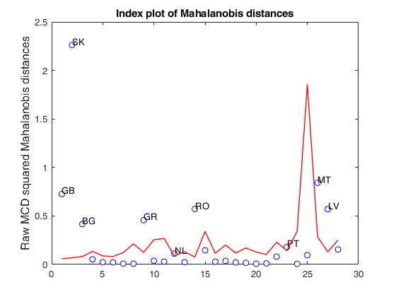
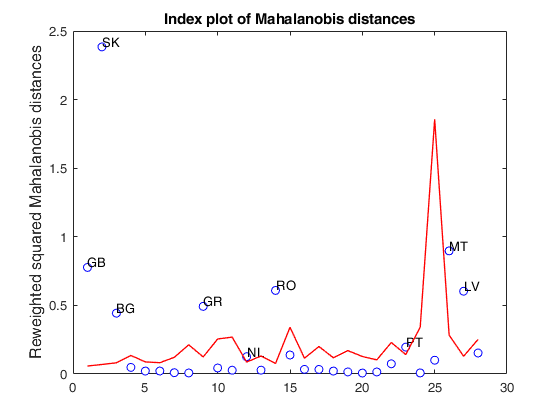
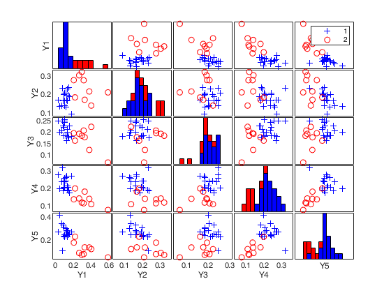
RAW=mcdCorAna(clothes,'plots',1,'findEmpiricalEnvelope',findEmp,'conflev',conflev);
Related Examples
 Example 2 of findEmpiricalEnvelope a struct
load clothes.
 Example 2 of findEmpiricalEnvelope a struct
load clothes.
Example 2 of findEmpiricalEnvelope a struct
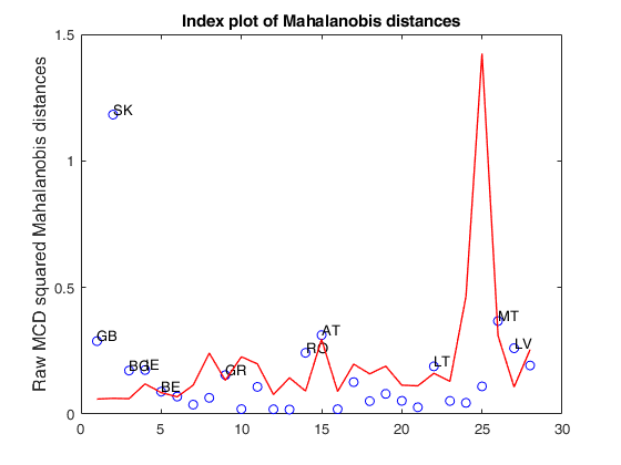
load clothes.load clothes.mat findEmp=struct; % Generate 500 contingency tables findEmp.nsimul=500; % Under the null hypothesis of independence findEmp.underH0=true; % Store the nsimul robust distances sorted (for each row) findEmp.StoreSim=true; % Detect outlying rows using a confidence level of 0.999 conflev=0.999; [RAW,REW]=mcdCorAna(clothes,'plots',1,'findEmpiricalEnvelope',findEmp,'conflev',conflev,'bdp',0.1);
Total estimated time to complete MCD:  0.02 seconds
Finding empirical bands

Input Arguments
N — Contingency table (default) or n-by-2 input dataset.
2D Array or Table.
2D array or table which contains the input contingency table (say of size I-by-J) or the original data matrix X.
In this last case N=crosstab(X(:,1),X(:,2)) or N=crosstab(X(:,1),X(:,2)) if X is in table format. As default procedure assumes that the input is a contingency table.
Data Types: table, or array
Name-Value Pair Arguments
Specify optional comma-separated pairs of Name,Value arguments.
Name is the argument name and Value
is the corresponding value. Name must appear
inside single quotes (' ').
You can specify several name and value pair arguments in any order as
Name1,Value1,...,NameN,ValueN.
 'bdp',1/4
, 'nsamp',10000
, 'refsteps',10
, 'reftol',1e-8
, 'refstepsbestr',10
, 'reftolbestr',1e-8
, 'bestr',10
, 'conflev',0.99
, 'plots',1
, 'Lr',{'UK' ...  'IT'}
, 'Lc',{'x1' ...  'x5'}
, 'msg',false
, 'tolMCD',1e-20
, 'findEmpiricalEnvelope',true
bdp
—Breakdown point.scalar.
(Number between 0 and 0.5) or if it an integer greater than 1 bdp is the number of data points which have to determine the fit The default value is 0.5.
Example: 'bdp',1/4
Data Types: double
nsamp
—Number of subsamples.scalar.
Number of subsamples of size J which have to be extracted (if not given, default = 1000).
Example: 'nsamp',10000
Data Types: double
refsteps
—Number of refining iterations.scalar.
Number of refining iterations in each subsample (default = 3).
refsteps = 0 means "raw-subsampling" without iterations.
Example: 'refsteps',10
Data Types: double
reftol
—Refining steps tolerance.scalar.
Tolerance for the refining steps.
The default value is 1e-6;
Example: 'reftol',1e-8
Data Types: double
refstepsbestr
—Number of refining iterations.scalar.
Number of refining iterations for each best subset (default = 50).
Example: 'refstepsbestr',10
Data Types: double
reftolbestr
—Tolerance for refining steps.scalar.
Value of tolerance for the refining steps for each of the best subsets.
The default value is 1e-8;
Example: 'reftolbestr',1e-8
Data Types: double
bestr
—Number of best solutions to store.scalar.
Number of "best locations" to remember from the subsamples. These will be later iterated until convergence (default=5)
Example: 'bestr',10
Data Types: double
conflev
—Confidence level.scalar.
Number between 0 and 1 containing confidence level which is used to declare units as outliers.
Usually conflev=0.95, 0.975 0.99 (individual alpha) or 1-0.05/I, 1-0.025/I, 1-0.01/I (simultaneous alpha).
Default value is 0.99 per cent simultaneous
Example: 'conflev',0.99
Data Types: double
plots
—Plot on the screen.scalar | structure.
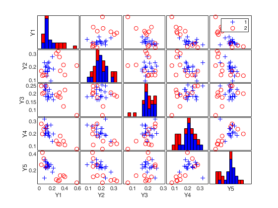
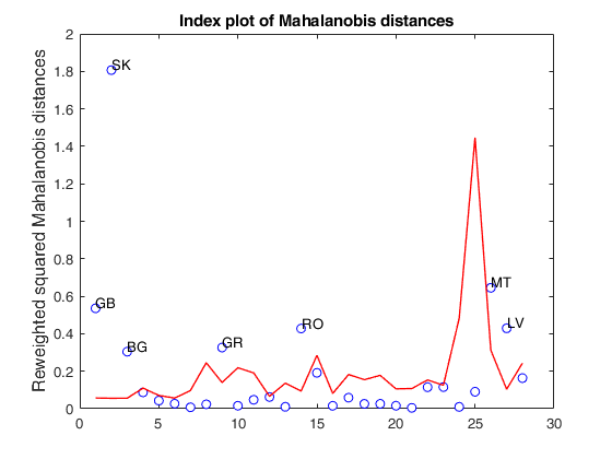
If plots is a structure or scalar equal to 1, generates: (1) a plot of Mahalanobis distances against index number. The confidence level used to draw the confidence bands for the MD is given by the input option conflev. If conflev is not specified a nominal 0.975 confidence interval will be used.
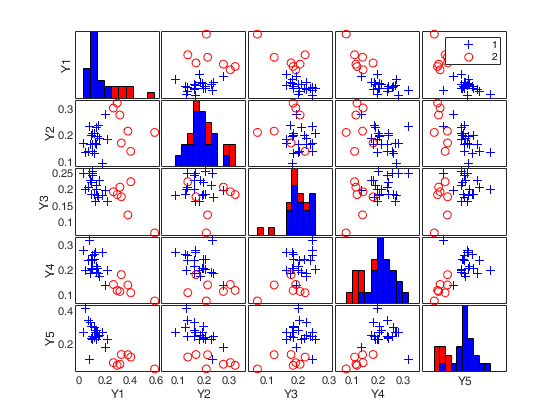
(2) a scatter plot matrix with the outliers highlighted.
If plots is a structure it may contain the following fields
| Value | Description |
|---|---|
labeladd |
if this option is '1', the outliers in the spm are labeled with their unit row index. The default value is labeladd='', i.e. no label is added. |
nameY |
cell array of strings containing the labels of the variables. As default value, the labels which are added are Y1, ...Yv. |
Example: 'plots',1
Data Types: double or structure
Lr
—row labels.cell array.
Cell of length I containing the labels of the rows.
Example: 'Lr',{'UK' ... 'IT'}
Data Types: cell
Lc
—column labels.cell array.
Cell of length J containing the labels of the columns.
Example: 'Lc',{'x1' ... 'x5'}
Data Types: cell
msg
—Display or not messages on the screen.boolean.
If msg==true (default) messages are displayed on the screen about estimated time to compute the final estimator else no message is displayed on the screen.
Example: 'msg',false
Data Types: logical
tolMCD
—Tolerance to declare a subset as singular.scalar.
The default value of tolMCD is exp(-50*v).
Example: 'tolMCD',1e-20
Data Types: double
findEmpiricalEnvelope
—Empirical Confidence level.boolean | struct.
If findEmpiricalEnvelope is true (default is false) the empirical envelope for each Mahalanobis distance of each Profile row of the contingency table is computed, else the empirical envelopes are found just if input option plots=1. In case findEmpiricalEnvelope is false the theoretical envelope is based on the quantiles of the following scaled gamma distribution chi2inv(conflev,(J-1)*(I-1)/I)/n,I,1)./r;
If findEmpiricalEnvelope is a struct it is possible to specify the following fields
| Value | Description |
|---|---|
nsimul |
number of simulations to compute the empirical envelope; |
underH0 |
boolean which specifies how to simulate the contingency tables. If findEmpiricalEnvelope.underH0=true the contingency tables are simulated under the null hypothesis of independence else they are simulated with a Chi2 value equal to the observed one based on all the observations (this value can be changed by field Chi2ValueToUse). |
Chi2ValueToUse |
positive scalar which specifies which Chi2 value to use to simulate the contingency tables. If this field is empty or is not present the value of Chi2 based on all n observations is used. Note that this option has an effect just if findEmpiricalEnvelope.underH0 is false. |
StoreSim |
boolean which specifies whether to store or not as fields named mdStore and NsimStore in output structs RAW and REW the sorted distances based on simulated contingency tables which have been generated and the simulated contingency tables. The default value of findEmpiricalEnvelope.StoreSimMD is false. |
Example: 'findEmpiricalEnvelope',true
Data Types: Boolean
Output Arguments
RAW — description
Structure
Structure which contains the following fields
| Value | Description |
|---|---|
h |
scalar. The number of observations that have determined the MCD estimator |
bdp |
scalar. The break down point of the MCD estimator |
loc |
1 x J vector containing raw MCD location of the data |
cov |
robust MCD estimate of covariance matrix. Note that RAW.cov is a diagonal matrix and on the main diagonal there is out.loc. |
obj |
The determinant of the raw MCD covariance matrix. |
bsb |
k x 1 vector containing the rows of matrix N which contributed to the computation of the MCD estimate of location |
md |
I x 1 vector containing the estimates of the robust Mahalanobis distances (in squared units). This vector contains the distances of each observation from the raw MCD location of the data, relative to the raw MCD scatter matrix diag(raw MCD location). Note that these distances are not multiplied by the masses. |
outliers |
A vector containing the list of the rows declared as outliers using confidence level specified in input scalar conflev. If no outlier is found RAW.outliers is empty. |
conflev |
Confidence level that was used to declare outliers and to do reweighting. |
singsub |
Number of subsets without full rank. Notice that out.singsub > 0.1*(number of subsamples) produces a warning |
weights |
I x 1 vector containing the estimates of the weights. Weights assume values in the interval [0 1]. Weight is 1 if the associated row fully contributes to compute centroid and covariance matrix. If for a particular row weight is 0.7 it means that the associated row contributes with 70 per cent of its row mass. 0 weight for a particular row it means that the associated row does not participate at all. Note that sum(N,2)'*RAW.weights=h |
N |
Original contingency table in array format. |
Ntable |
Original contingency table in table format. |
Y |
array I-by-J containing matrix of Profile Rows. |
EmpEnv |
array of size I-by-1 containing empirical envelopes for each Mahalanobis distance if input option findEmpiricalEnvelope is true or scalar containing quantile which has been used to declare the outliers. |
simulateUnderH0 |
is boolean. It is true if the simulated contingency tables have been specified under H0. |
mdStore |
array of size I-by-nsimul which contains the robust squared Mahalanobis distances for each row of the contingency table across the nsimul simulations based on simulated contingency tables. The rows are ordered in ascending order. This output is present just if input option findEmpiricalEnvelope is a struct and findEmpiricalEnvelope.StoreSimMD is true. Note that the these squared MD are not multiplied by masses. |
NsimStore |
array of size IxJ-by-nsimul which contains the simulated contingency tables. First column contains the first contingency table stored in vector format... This output is present just if input option findEmpiricalEnvelope is a struct and findEmpiricalEnvelope.StoreSim is true. |
class |
'mcdCorAna' |
REW — description
Structure
Structure which contains the following fields
| Value | Description |
|---|---|
N |
Original contingency table in array format. |
Ntable |
Original contingency table in table format. |
md |
I x 1 vector containing the estimates of the robust Mahalanobis distances (in squared units). This vector contains the distances of each observation from the reweighted MCD location of the data, relative to the reweighted MCD scatter matrix diag(reweighted MCD location) |
h |
scalar. The number of observations that have determined the MCD estimator |
weights |
I x 1 vector containing the estimates of the weights. Weights assume values 0 or 1. Weight is 0 if the associated row has been declared outlier after reweighting. |
outliers |
A vector containing the list of the rows declared as outliers using confidence level specified in input scalar conflev |
Y |
array I-by-J containing matrix of Profile Rows. |
EmpEnv |
array of size I-by-1 containing empirical envelopes for each Mahalanobis distance if input option findEmpiricalEnvelope is true or scalar containing quantile which have been used to declare the outliers. |
mdStore |
array of size I-by-nsimul which contains the robust Mahalanobis distances for each row of the contingency table across the nsimul simulations based on simulated contingency tables. The rows are ordered in ascending order. This output is present just if input option findEmpiricalEnvelope is a struct and findEmpiricalEnvelope.StoreSimMD is true. |
class |
'mcdCorAna' |
varargout —Indices
of the subsamples extracted for
computing the estimate.
C : matrix of size nsamp-by-J
More About
Additional Details
MCDcorAna computes the MCD estimator for a contingency table. This estimator is given by the subset of s Profile rows with smallest covariance determinant. The MCD location estimate is then the mean of those h Profile points.
The default value of h is roughly 0.5n (where n is the total number of observations), but the user may choose each value between n/2 and n.
References
Greenacre, M.J. (1993), "Correspondence Analysis in Practice", London, Academic Press.
Riani, M, Atkinson A.C., Torti, F., Corbellini A. (2023), Robust Correspondence Analysis, "Journal of the Royal Statistical Society Series C: Applied Statistics", Vol. 71, pp. 1381–1401, https://doi.org/10.1111/rssc.12580
