ellipse
ellipse generates an ellipse given mu (location vector) and Sigma (scatter matrix)
Syntax
Description
The ellipse is generated using the equation: \[ (x-\mu)' \Sigma^{-1} (x-\mu) = c_{conflev}^2. \] The length of the i-th principal semiaxis $(i=1, 2)$ is $c_{conflev} \sqrt \lambda_i$ where $\lambda_i$ is the $i$-th eigenvalue of $\Sigma$.
Examples
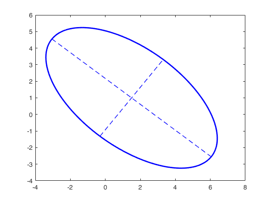
 Draw the ellipse using a blue color line.
Draw the ellipse using a blue color line.
close all
rho=-2;
A=[4 rho; rho 3 ];
mu=[1.5 1];
Color=[0 0 1];
ellipse(mu,A,[],Color);
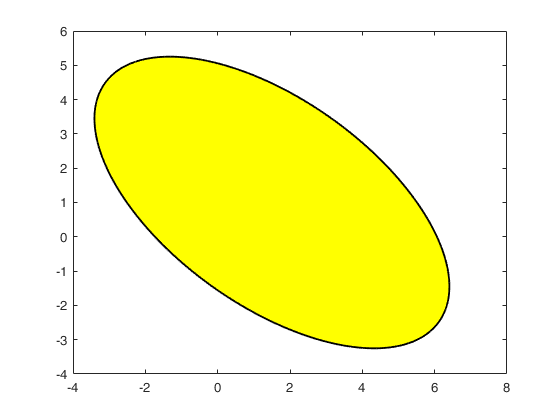
Draw an ellipse and fill it with yellow color.
Draw an ellipse and fill it with yellow color.
close all
rho=-2;
A=[4 rho; rho 3 ];
mu=[1.5 1];
Ell=ellipse(mu,A);
patch(Ell(:,1),Ell(:,2),'y');
99 per cent confidence ellipse.
99 per cent confidence ellipse.Generate 1000 bivariate normal data and add the ellipse which contains approximately 990 of them.
rng('default')
rng(20)     % For reproducibility
% Define mu and Sigma
mu = [2,3];
Sigma = [1,1.5;1.5,3];
Y = mvnrnd(mu,Sigma,1000);
figure
hold on;
plot(Y(:,1),Y(:,2),'o');
% add an ellipse to these points
Ell=ellipse(mu,Sigma,0.99);
axis equal
% Count number of points inside the ellipse
disp('Number of points inside the ellipse')
disp(sum(inpolygon(Y(:,1),Y(:,2),Ell(:,1),Ell(:,2))))
Number of points inside the ellipse 987

Input Arguments
Output Arguments
References
Mardia, K.V., J.T. Kent, and J.M. Bibby (1979), "Multivariate Analysis," Academic Press, London, p. 140. [MKB].