histFS
histFS plots a histogram with the elements in each bin grouped according to a vector of labels.
Syntax
Description
Examples
 An example with 4 groups.
An example with 4 groups.
close all;
y = randn(500,1);
% four groups
groups = randi(4,500,1);
% number of bins
nbins = 10;
[ng, hb] = histFS(y,nbins,groups);
title('Histogram with default color rotation (brcmykg)','interpreter','latex','FontSize',18);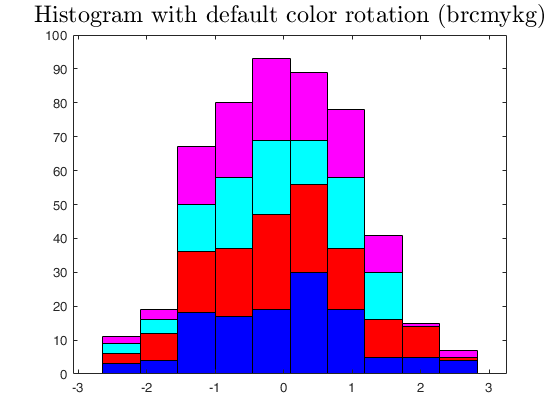
The same histogram is now plotted with different legends.
The same histogram is now plotted with different legends.
figure;
y = randn(500,1);
groups = randi(4,500,1);
nbins = 10;
% 4th positional input argument is the legend labels.
[ng, hb] = histFS(y,nbins,groups,{'BMW','FIAT','VOLVO','FERRARI'});
title('The same, with personalized legends','interpreter','latex','FontSize',18);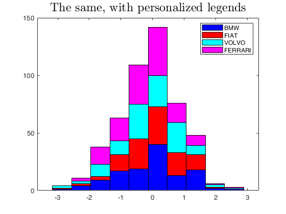
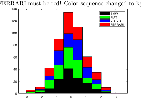
The same histogram is now plotted with different colors.
The same histogram is now plotted with different colors.
figure;
y = randn(500,1);
groups = randi(4,500,1);
nbins = 10;
% 6th positional input argument is the colors
[ng, hb] = histFS(y,nbins,groups,{'BMW','FIAT','VOLVO','FERRARI'},gca,'kgbr');
title('FERRARI must be red! Color sequence changed to kgbr','interpreter','latex','FontSize',18);
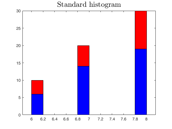
Example of weighted histogram.
Example of weighted histogram.
close all;clear all;
X = crosstab2datamatrix([10 20 30]); X=X(:,2);
X1 = 444*ones(60,1); X1(40:60)= 999; X1 = shuffling(X1);
X = X+5;
if verLessThan('matlab','8.5')
groups = num2str(X1);
else
groups = categorical(X1);
end
W = ones(size(X,1),1); W(12) = 100;
histFS(X,10,groups,[],[],[],W);
title({'Weighted histograms:' , 'please check with tabulateFS(W) and tabulateFS(X)'},'interpreter','latex','FontSize',18);
figure;
histFS(X,10,groups);
title('Standard histogram','interpreter','latex','FontSize',18);
cascade;
disp('tabulateFS(X)');
tabulateFS(X);
disp('tabulateFS(W)');
tabulateFS(W);
tabulateFS(X)
6 10 16.67%
7 20 33.33%
8 30 50.00%
tabulateFS(W)
1 59 98.33%
100 1 1.67%
Related Examples
Example of second input argument a vector containing the edges.
Example of second input argument a vector containing the edges.
load citiesItaly.mat
zone=[repelem("N",46) repelem("CS",57)]';
edges=[0 15000:5000:35000];
lege={'CS' 'N'};
freq1=histFS(citiesItaly.addedval,edges,zone,lege);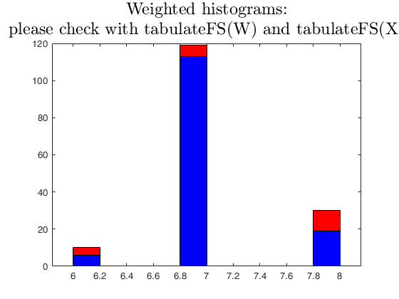
Input Arguments
Output Arguments
References
Tufte E.R. (1983), "The visual display of quantitative information", Graphics Press, Cheshire.