inversegampdf
inversegampdf computes inverse-gamma probability density function.
Description
Examples
 Plot the pdf for 4 different combinations of parameter values.
Plot the pdf for 4 different combinations of parameter values.
x=(0:0.001:3)';
a=[1,2,3,3];
b=[1,1,1,0.5];
for j=1:4
subplot(2,2,j);
plot(x,inversegampdf(x,a(j),b(j)));
xlabel('x');
title(['PDF with a=' num2str(a(j)) ' b=' num2str(b(j))]);
end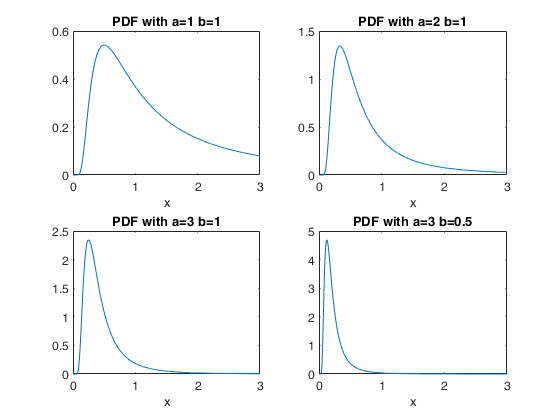
Compare the results using option nocheck=1.
Compare the results using option nocheck=1.
x=(0:0.001:3)';
a=[1,2,3,50,100,10000];
b=[1,10,100,0.05,10,800];
Y=zeros(length(x),length(a));
Ychk=Y;
for i=1:length(x)
Y(i,:)   = inversegampdf(x(i),a,b);
Ychk(i,:)= inversegampdf(x(i),a,b,1);
end
disp('Maximum absolute difference is:');
disp(max(max(abs(Y-Ychk))));
Maximum absolute difference is:
0.00
Related Examples
Interpretation in Bayesian statistics.
Interpretation in Bayesian statistics.Interpretation of a inverse Gamma (conjugate) prior, used for estimating the posterior distribution of the unknown variance $\sigma{^2}$ of a normal $N(0,\sigma{^2})$.
% a set of values for $\sigma^2$
x=(0:0.001:3)';
% Two panels with inverse Gamma distribution for different parameters
% settings.
% Left panel:  fixed shape (1), increasing scale (1,2,4);
% As the scale parameter increases, the mean of the distribution (more
% and more skewed to the right) also increases. This suggests that an
% inverse Gamma prior with a larger scale parameter incorporates a prior
% belief in favour of a larger value for $\sigma^2$.
a = [1, 1, 1];
b = [1, 2, 4];
subplot(1,2,1);
for j=1:3
plot(x,inversegampdf(x,a(j),b(j)));
hold on;
xlabel('x (\sigma^2)');
end
title('PDF with a=[1, 1, 1] and b=[1, 2, 4]');
% Right panel: fixed scale (1), increasing shape (1,2,4);
% As the shape parameter increases, the distribution becomes more and
% more centered around the mean, producing a tighter set of prior beliefs.
b = [1, 1, 1];
a = [1, 2, 4];
subplot(1,2,2);
for j=1:3
plot(x,inversegampdf(x,a(j),b(j)));
hold on;
xlabel('x (\sigma^2)');
end
title('PDF with a=[1, 2, 4] and b=[1, 1, 1]');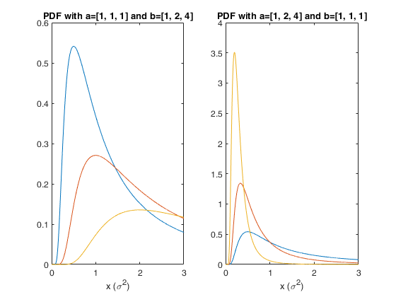
Input Arguments
Output Arguments
More About
References
Zellner, A. (1971), "An introduction to Bayesian Inference in Econometrics", Wiley.
[ https://en.wikipedia.org/wiki/Inverse-gamma_distribution ]