kdebiv
kdebiv computes (and optionally plots) a kernel smoothing estimate for bivariate data.
Syntax
Description
This function is introduced in FSDA to support MATLAB releases older than R2016a, when function ksdensity was only addressing one-dimensional data.
For R2016a and subsequent releases, kdebiv uses ksdensity. Otherwise, the function computes a nonparametric estimate of the probability density function based on a normal kernel and using a bandwidth estimated as a function of the number of points in X.
An example using colormap.F
=kdebiv(X,
Name, Value)
Examples
 Density plots for a mixture of two normal distributions.
Density plots for a mixture of two normal distributions.
X1 = [0+.5*randn(150,1)   5+2.5*randn(150,1)];
X2 = [1.75+.25*randn(60,1) 8.75+1.25*randn(60,1)];
X = [X1 ; X2];
% A filled contour plot obtained using colormap 'cmap' = 'summer'.
[F1,Xi,bw] = kdebiv(X,'contourtype','contourf','cmap','summer');
title('A filled contour plot obtained using colormap ''summer''');
hold on
plot(X(:,1),X(:,2),'rx')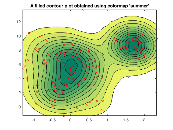
Related Examples
Input Arguments
Output Arguments
References
Bowman, A.W. and Azzalini, A. (1997), "Applied Smoothing Techniques for Data Analysis", Oxford University Press.