logmvnpdfFS

logmvnpdfFS produces log of Multivariate normal probability density function (pdf)

Syntax

  • y=logmvnpdfFS(X, Mu, Sigma)example
  • y=logmvnpdfFS(X, Mu, Sigma, X0)example
  • y=logmvnpdfFS(X, Mu, Sigma, X0, eyed)example
  • y=logmvnpdfFS(X, Mu, Sigma, X0, eyed, n)example
  • y=logmvnpdfFS(X, Mu, Sigma, X0, eyed, n, d)example
  • y=logmvnpdfFS(X, Mu, Sigma, X0, eyed, n, d, msg)example
  • y=logmvnpdfFS(X, Mu, Sigma, X0, eyed, n, d, msg, callmex)example

Description

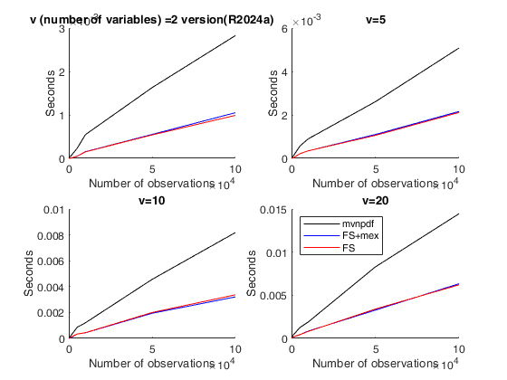
This function is a much faster version than (log of) Matlab function mvnpdf. If this function is called without optional arguments than it uses matlab function bsxfun to compute the deviations form the means and no mex function.

If this function is called with the four optional input arguments X0, eyed, n and d a mex function based on C code is directly used.

Additional details follow: in order to compute the kernel of the quadratic form at the exponent logmvnpdfFS creates an identity of size length(Mu) and similarly needs to compute length(Mu). These two quantites can be precalculated and supplied as input parameters. If logmvnpdfFS has to be called thousands of times (as it happens for example in each iteration of all procedures of cluster analysis based mixtures of multivariate gaussian distributions). The same argument above applies to scalars n and d which are directly passed to the compiled mex function

example

y =logmvnpdfFS(X, Mu, Sigma) Call to logmvnpdfFS with 3 input arguments.

example

y =logmvnpdfFS(X, Mu, Sigma, X0) Comparison with mvnpdf.

example

y =logmvnpdfFS(X, Mu, Sigma, X0, eyed) Remark: Options X0, eyed, n, and d must be used together.

example

y =logmvnpdfFS(X, Mu, Sigma, X0, eyed, n) TIME COMPARISON USING TIC TOC.

example

y =logmvnpdfFS(X, Mu, Sigma, X0, eyed, n, d) TIME COMPARISON USING TIMEIT FUNCTION.

example

y =logmvnpdfFS(X, Mu, Sigma, X0, eyed, n, d, msg) Example of the use of option msg 0.

example

y =logmvnpdfFS(X, Mu, Sigma, X0, eyed, n, d, msg, callmex) Example of the use of option msg 1.

Examples

expand all

  • Call to logmvnpdfFS with 3 input arguments.
  • n=20;
    v=2;
    X=randn(n,v);
    mu = [1 1]; Sigma = [.9 .4; .4 .3];
    y = logmvnpdfFS(X, mu, Sigma);

  • Comparison with mvnpdf.
  • In this example we check the agreement of the results with MATLAB function mvnpdf.

    n=20000;
    v=2;
    X=randn(n,v);
    mu = [1 -1]; Sigma = [.9 .4; .4 .3];
    y = logmvnpdfFS(X, mu, Sigma);
    y1=log(mvnpdf(X,mu,Sigma));
    max(abs(y-y1))
    % 2.842e-14

  • TIME COMPARISON USING TIC TOC.
  • In the examples below we compare the speed of the different solutions logmvnpdfFS with mex function and logmvnpdfFS without mex function

    % In this code computation time is based on tic toc combined with a series
    % of replications
    % nn = sample size
    % vv = number of variables
    nn=[100 200 500 1000 5000 10000 50000 100000];
    vv=[2 5 10 20];
    % rep =number of replications
    rep = 1000;
    ttMat=nan(length(nn) , length(vv));
    ttFSwithMex=ttMat;
    ttFSnoMex=ttMat;
    Mat=0; tMat=0;
    FSwithmex=0; tFSwithMex=0;
    FSnoMex=0; tFSnoMex=0;
    in = 1; iv=1;
    for n = nn
    for v = vv
    X0 = zeros(n,v);
    eyed=eye(v);
    for i=1:rep
    X = randn(n,v);
    Mu = randn(1,v);
    Sigma=cov(X);
    %  Matlab function mvnpdf, (black line in plot)
    Mat = tic;
    y0 = mvnpdf(X, Mu, Sigma);
    y0=log(y0);
    tMat = tMat + toc(Mat);
    % logmvnpdfFS using mex file for mean deviations, (blue line in plot)
    FSwithmex = tic;
    yD = logmvnpdfFS(X, Mu, Sigma,X0,eyed,n,v);
    tFSwithMex = tFSwithMex + toc(FSwithmex);
    % logmvnpdfFS and no mex file for mean deviations. (red line in plot)
    FSnoMex = tic;
    yI = logmvnpdfFS(X, Mu, Sigma);
    tFSnoMex = tFSnoMex + toc(FSnoMex);
    if (sum(sum(abs(y0-yD))))>10^-6  || (sum(sum(abs(y0-yI)))) >10^-6
    error('FSDA:logmvnpdfFS:ShouldBeEq','Difference in results: stop');
    end
    end
    ttMat(in,iv) = tMat;
    ttFSwithMex(in,iv) = tFSwithMex;
    ttFSnoMex(in,iv) = tFSnoMex;
    Mat=0; tMat=0;
    FSwithmex=0; tFSwithMex=0;
    FSnoMex=0; tFSnoMex=0;
    disp(['n=' num2str(n) ' -- v=' num2str(v)]);
    iv = iv+1;
    end
    in = in+1;
    iv = 1;
    end
    % Plotting part
    a=ver;
    a=a.Release;
    aa=1;
    bb=8;
    for ij=1:length(vv);
    subplot(length(vv)/2,2,ij)
    hold('on')
    plot(nn(aa:bb)',ttMat(aa:bb,ij),'k');
    plot(nn(aa:bb)',ttFSwithMex(aa:bb,ij),'b')
    plot(nn(aa:bb)',ttFSnoMex(aa:bb,ij),'r');
    if ij==1
    title(['v (number of variables)=' num2str(vv(ij)) ' version' a])
    else
    title(['v=' num2str(vv(ij))])
    end
    ylabel('Seconds')
    xlabel('Number of observations')
    if ij==4
    legend('mvnpdf','FS+mex','FS','location','NorthWest')
    end
    end
    hold off;

  • TIME COMPARISON USING TIMEIT FUNCTION.
  • Remark: timeit function is present from MATLAB 2013b

    if verLessThan('matlab', '8.2.0')
    warning('FSDA:logmvnpdfFS:MatlabTooOld','This example needs routine timeit which has been introduced in Matlab 2013b')
    warning('FSDA:logmvnpdfFS:MatlabTooOld','You have a version of Matlab which is < 2013b and you cannot run this example')
    else
    % nn = sample size
    % vv = number of variables
    nn=[100 200 500 1000 5000 10000 50000 100000];
    vv=[2 5 10 20];
    ttMat=nan(length(nn) , length(vv));
    ttFSwithMex=ttMat;
    ttFSnoMex=ttMat;
    in = 1; iv=1;
    for n = nn
    for v = vv
    X0 = zeros(n,v);
    eyed=eye(v);
    X = randn(n,v);
    Mu = randn(1,v);
    Sigma=cov(X);
    %  Matlab function mvnpdf
    yMat = @() log(mvnpdf(X, Mu, Sigma));
    tMat = timeit(yMat);
    % logmvnpdfFS using mex file for mean deviations.
    yFSwithMex = @() logmvnpdfFS(X, Mu, Sigma,X0,eyed,n,v);
    tFSwithMex = timeit(yFSwithMex);
    % logmvnpdfFS and no mex file for mean deviations.
    yFSnoMex = @() logmvnpdfFS(X, Mu, Sigma);
    tFSnoMex = timeit(yFSnoMex);
    ttMat(in,iv) = tMat;
    ttFSwithMex(in,iv) = tFSwithMex;
    ttFSnoMex(in,iv) = tFSnoMex;
    disp(['n=' num2str(n) ' -- v=' num2str(v)]);
    iv = iv+1;
    end
    in = in+1;
    iv = 1;
    end
    % Plotting part
    a=ver;
    a=a.Release;
    aa=1;
    bb=length(nn);
    for ij=1:length(vv);
    subplot(length(vv)/2,2,ij)
    hold('on')
    plot(nn(aa:bb)',ttMat(aa:bb,ij),'k');
    plot(nn(aa:bb)',ttFSwithMex(aa:bb,ij),'b')
    plot(nn(aa:bb)',ttFSnoMex(aa:bb,ij),'r');
    if ij==1
    title(['v (number of variables) =' num2str(vv(ij)) ' version' a])
    else
    title(['v=' num2str(vv(ij))])
    end
    xlabel('Number of observations')
    ylabel('Seconds')
    if ij==4
    legend('mvnpdf','FS+mex','FS','location','NorthWest')
    end
    end
    hold off;
    end
    n=100 -- v=2
    n=100 -- v=5
    n=100 -- v=10
    n=100 -- v=20
    n=200 -- v=2
    n=200 -- v=5
    n=200 -- v=10
    n=200 -- v=20
    n=500 -- v=2
    n=500 -- v=5
    n=500 -- v=10
    n=500 -- v=20
    n=1000 -- v=2
    n=1000 -- v=5
    n=1000 -- v=10
    n=1000 -- v=20
    n=5000 -- v=2
    n=5000 -- v=5
    n=5000 -- v=10
    n=5000 -- v=20
    n=10000 -- v=2
    n=10000 -- v=5
    n=10000 -- v=10
    n=10000 -- v=20
    n=50000 -- v=2
    n=50000 -- v=5
    n=50000 -- v=10
    n=50000 -- v=20
    n=100000 -- v=2
    n=100000 -- v=5
    n=100000 -- v=10
    n=100000 -- v=20
    
    Click here for the graphical output of this example (link to Ro.S.A. website).

  • Example of the use of option msg 0.
  • n=20000;
    v=2;
    X=randn(n,v);
    mu = [1 -1]; Sigma = [.9 1; 1 .3];
    msg=0;
    X0=X;
    eyed=eye(v);
    y = logmvnpdfFS(X,mu,Sigma,X0,eyed,n,v,msg);
    % y is -Inf but no warning is shown.

  • Example of the use of option msg 1.
  • n=20000;
    v=2;
    X=randn(n,v);
    mu = [1 -1]; Sigma = [.9 1; 1 .3];
    msg=1;
    X0=X;
    eyed=eye(v);
    y = logmvnpdfFS(X,mu,Sigma,X0,eyed,n,v,msg);
    %  y is -Inf and warning is shown.

    Input Arguments

    expand all

    X — Input data. Scalar, Vector or matrix.

    n x d data matrix; n observations and d variables. Rows of Y represent observations, and columns represent variables or coordinates.

    The (log of the) probability density of the multivariate normal distribution will be evaluated at each row of the n-by-d matrix Y

    Data Types: single|double

    Mu — mean mu of the multivariate normal distribution. 1-by-d vector.

    Data Types: single|double

    Optional Arguments

    X0 — matrix of the same size of X which passes to C function a container. Note that options X0, eyed, n, and d must be supplied together.

    Example: 'X0',X

    Data Types: single|double

    eyed — identity matrix of size length(Mu) wchich passes to C function a container. Note that options X0, eyed, n, and d must be supplied together.

    Example: 'eyed',eye(v)

    Data Types: single|double

    n — scalar which passes to C function size(X,1). Note that options X0, eyed, n, and d must be supplied together.

    Example: 'eyed',eye(v)

    Data Types: single|double

    d — scalar which passes to C function length(Mu). Note that options X0, eyed, n, and d must be supplied together.

    Example: 'eyed',eye(v)

    Data Types: single|double

    msg — Level of output to display. Scalar.

    Scalar which controls whether to display or not messages on the screen. If msg==1 (default) messages are displayed on the screen when cholesky of Sigma is impossibile else no message is displayed on the screen. When Clolesky of Sigma is impossible -Inf output is returned.

    Example: 'msg',1

    Data Types: single | double

    callmex — call or not mex function to compute the result. Boolean.

    Boolean which controls whether to call or not the mex function.

    Example: 'callmex',false

    Data Types: boolean

    Output Arguments

    expand all

    y —log-density of the multivariate normal. Vector

    Vector with length equal to n which returns the log-density of the multivariate normal distribution with mean Mu and covariance Sigma, evaluated at each row of X.

    References

    See Also

    This page has been automatically generated by our routine publishFS