mdrplot
mdrplot plots the trajectory of minimum deletion residual (mdr)
Syntax
Description
Example of the use of function mdrplot with all the default options.brushedUnits
=mdrplot(out)
Example of the use of function mdrplot with personalized envelopes.brushedUnits
=mdrplot(out,
Name, Value)
[
datatooltip passed as scalar.brushedUnits,
BrushedUnits]
=mdrplot(___)
Examples
Example of the use of function mdrplot with all the default options.
Steps common to all the examples
load('loyalty.txt','loyalty');
y=loyalty(:,4);
X=loyalty(:,1:3);
[outLXS]=LXS(y,X,'nsamp',1000);
[out]=FSReda(y,X,outLXS.bs);
mdrplot(out);
Example of the use of function mdrplot with personalized envelopes.
load('loyalty.txt','loyalty');
y=loyalty(:,4);
X=loyalty(:,1:3);
[outLXS]=LXS(y,X,'nsamp',1000);
[out]=FSReda(y,X,outLXS.bs);
mdrplot(out,'quant',[0.99;0.9999]);
datatooltip passed as scalar.
Example of the use of function mdrplot with datatooltip passed as scalar (that is using default options for datacursor (i.e.
%DisplayStyle =window)
load('loyalty.txt','loyalty');
y=loyalty(:,4);
X=loyalty(:,1:3);
[outLXS]=LXS(y,X,'nsamp',1000);
[out]=FSReda(y,X,outLXS.bs);
mdrplot(out,'datatooltip',1);
Related Examples
Datatooltip passed as structure.
load('loyalty.txt','loyalty');
y=loyalty(:,4);
X=loyalty(:,1:3);
[outLXS]=LXS(y,X,'nsamp',1000);
[out]=FSReda(y,X,outLXS.bs);
clear tooltip
tooltip.SnapToDataVertex='on'
tooltip.DisplayStyle='datatip'
mdrplot(out,'datatooltip',tooltip);
Use of option sign.
Example of the information which can be extracted from option sign=1 (default). If the data come from a distribution which has positive asymmetry generally the last part of the search is associated with positive values of the minimum residual among the units belonging to subset The example below shows that the last 60 steps of the curve are associated with a black curve (positive value of mdr)
state = 137; state1=4567;
rand('state', state);
randn('state', state1);
X=randn(200,3);
y=chi2rnd(8,200,1);
[outLXS]=LXS(y,X,'nsamp',1000);
[out]=FSReda(y,X,outLXS.bs);
mdrplot(out,'sign',1);
Example of the use of option envm.
In this case the resuperimposed envelope is based on n-2 observations
state = 137; state1=4567;
rand('state', state);
randn('state', state1);
X=randn(200,3);
y=chi2rnd(8,200,1);
[outLXS]=LXS(y,X,'nsamp',1000);
[out]=FSReda(y,X,outLXS.bs);
mdrplot(out,'envm',length(out.y)-2);
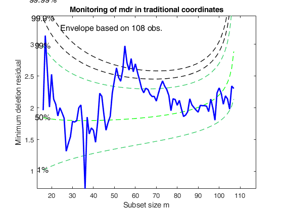
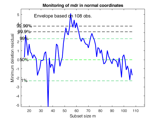
 Example of the use of option ncoord.
Example of the use of option ncoord.In this example we compare the monitoring residual plot in traditional coordinates with that in normal coordinates.
% load the Hospital data
load('hospitalFS.txt');
y=hospitalFS(:,5);
X=hospitalFS(:,1:4);
% Set initial subset
bs= [ 3   11   20   23   74];
outFS=FSReda(y,X,bs);
p=size(X,2)+1;
quant=[0.01 0.5 0.99 0.999 0.9999];
mdrplot(outFS,'quant',quant,'tag','mdrorigcooed')
title('Monitoring of mdr in traditional coordinates')
% Transform the values of mdr into normal coordinates
[MDRinv] = FSRinvmdr(abs(outFS.mdr),p);
outFS1=outFS;
outFS1.mdr=MDRinv(:,[1 3]);
mdrplot(outFS1,'ncoord',true,'quant',quant,'tag','mdrncoord')
title('Monitoring of mdr in normal coordinates')
ans =

     []


ans =

     []
Interactive example 1.
Input option databrush passed as scalar.
%Example of the use of function mdrplot with databrush
state = 137; state1=4567;
rand('state', state);
randn('state', state1);
X=randn(200,3);
y=chi2rnd(8,200,1);
[outLXS]=LXS(y,X,'nsamp',1000);
[out]=FSReda(y,X,outLXS.bs);
mdrplot(out,'databrush',1);
Interactive example 2.
Input option databrush passed as structure.
%Example where databrush is a structure
state = 137; state1=4567;
rand('state', state);
randn('state', state1);
X=randn(200,3);
y=chi2rnd(8,200,1);
[outLXS]=LXS(y,X,'nsamp',1000);
[out]=FSReda(y,X,outLXS.bs);
databrush=struct
databrush.selectionmode='Lasso'
mdrplot(out,'databrush',databrush)
Interactive example 3.
Input option databrush passed as structure and brush mode.
%Example of the use of brush using brush mode
state = 137; state1=4567;
rand('state', state);
randn('state', state1);
X=randn(200,3);
y=chi2rnd(8,200,1);
[outLXS]=LXS(y,X,'nsamp',1000);
[out]=FSReda(y,X,outLXS.bs);
databrush=struct
databrush.selectionmode='Brush'
databrush.Label='on';
mdrplot(out,'databrush',databrush)
Interactive example 4.
Persistent cumulative brush 1.
%Example of the use of persistent non cumulative brush. Every time a
%brushing action is performed previous highlightments are removed
state = 137; state1=4567;
rand('state', state);
randn('state', state1);
X=randn(200,3);
y=chi2rnd(8,200,1);
[outLXS]=LXS(y,X,'nsamp',1000);
[out]=FSReda(y,X,outLXS.bs);
databrush=struct
databrush.persist='off'
databrush.RemoveLabels='off';
mdrplot(out,'databrush',databrush)
Interactive example 5.
Persistent cumulative brush 2.
%Example of the use of persistent cumulative brush. Every time a
%brushing action is performed current highlightments are added to
%previous highlightments
state = 137; state1=4567;
rand('state', state);
randn('state', state1);
X=randn(200,3);
y=chi2rnd(8,200,1);
[outLXS]=LXS(y,X,'nsamp',1000);
[out]=FSReda(y,X,outLXS.bs);
databrush=struct
databrush.persist='on';
databrush.selectionmode='Rect'
% outV is the vector of all selected units during brushing
% outM is a matrix, each column contains the groups of selected units
% at each brushing action
[outV, outM]=mdrplot(out,'databrush',databrush)
Input Arguments
out — Structure containing monitoring of mdr.
Structure.
Structure containing the following fields.
| Value | Description |
|---|---|
mdr |
minimum deletion residual. A matrix containing the monitoring of minimum deletion residual in each step of the forward search. The first column of mdr must contain the fwd search index This matrix can be created using function FSReda (compulsory argument) |
Un |
order of entry of each unit. Matrix containing the order of entry of each unit (necessary if datatooltip is true or databrush is not empty) |
y |
response. Vector containing the response (necessary only if option databrush is not empty) |
X |
Regressors. A matrix containing the explanatory variables (necessary only if option databrush is not empty) |
Bols |
Monitoring of beta coefficients. (n-init+1) x (p+1) matrix containing the monitoring of estimated beta coefficients in each step of the forward search (necessary only if option databrush is not empty and suboption multivarfit is not empty) |
Data Types: single|double
Name-Value Pair Arguments
Specify optional comma-separated pairs of Name,Value arguments.
Name is the argument name and Value
is the corresponding value. Name must appear
inside single quotes (' ').
You can specify several name and value pair arguments in any order as
Name1,Value1,...,NameN,ValueN.
 'quant',[0.05;0.5;0.95]
, 'sign',1
, 'mplus1',1
, 'envm',100
, 'xlimx',[20 100]
, 'ylimy',[2 6]
, 'lwdenv',2
, 'ncoord',true
, 'tag','mymdr'
, 'datatooltip',''
, 'label',{'Smith','Johnson','Robert','Stallone'}
, 'databrush',1
, 'FontSize',14
, 'SizeAxesNum',14
, 'nameX',{'Age','Income','Married','Profession'}
, 'namey','response label'
, 'lwd',3
, 'namey','Plot title'
, 'labx','Subset size m'
, 'laby','mdr'
quant
—Quantiles for which envelopes have
to be computed.vector.
The default is to produce 1%, 50% and 99% envelopes. In other words the default is quant=[0.01;0.5;0.99];
Example: 'quant',[0.05;0.5;0.95]
Data Types: double
sign
—mdr with sign.scalar.
If it is equal 1 (default) we distinguish steps for which minimum deletion residual was associated with positive or negative value of the residual. Steps associated with positive values of mdr are plotted in black, while other steps are plotted in red.
Example: 'sign',1
Data Types: double
mplus1
—plot of (m+1)th order statistic.scalar.
Scalar, which specifies if it is necessary to plot the curve associated with (m+1)th order statistic.
Example: 'mplus1',1
Data Types: double
envm
—sample size for drawing envelopes.scalar.
Scalar which specifies the size of the sample which is used to superimpose the envelope. The default is to add an envelope based on all the observations (size n envelope).
Example: 'envm',100
Data Types: double
xlimx
—min and max for x axis.vector.
vector with two elements controlling minimum and maximum on the x axis.
Default value is mdr(1,1)-3 and mdr(end,1)*1.3
Example: 'xlimx',[20 100]
Data Types: double
ylimy
—min and max for x axis.vector.
Vector with two elements controlling minimum and maximum on the y axis.
Default value is min(mdr(:,2)) and max(mdr(:,2));
Example: 'ylimy',[2 6]
Data Types: double
lwdenv
—Line width.scalar.
Scalar which controls the width of the lines associated with the envelopes.
Default is lwdenv=1
Example: 'lwdenv',2
Data Types: double
ncoord
—input out.mdr in normal coordinates.
Boolean.
If ncoord=true the input matrix which contains the minimum deletion residual has been transformed to normal coordinates. The default is ncoord false.
Example: 'ncoord',true
Data Types: logical
tag
—plot handle.string.
String which identifies the handle of the plot which is about to be created. The default is to use tag 'pl_mdr'. Notice that if the program finds a plot which has a tag equal to the one specified by the user, then the output of the new plot overwrites the existing one in the same window else a new window is created.
Example: 'tag','mymdr'
Data Types: char
datatooltip
—interactive clicking.empty value (default) | structure.
If datatooltip is not empty the user can use the mouse in order to have information about the unit selected, the step in which the unit enters the search and the associated label. If datatooltip is a structure, it is possible to control the aspect of the data cursor (see function datacursormode for more details or the examples below). The default options of the structure are DisplayStyle='Window' and SnapToDataVertex='on'
Example: 'datatooltip',''
Data Types: empty value, numeric or structure
label
—row labels.cell of strings.
Cell containing the labels of the units (optional argument used when datatooltip=1. If this field is not present labels row1, ..., rown will be automatically created and included in the pop up datatooltip window)
Example: 'label',{'Smith','Johnson','Robert','Stallone'}
Data Types: cell
databrush
—interactive mouse brushing.empty value (default), scalar | structure.
DATABRUSH IS AN EMPTY VALUE.
If databrush is an empty value (default), no brushing is done. The activation of this option (databrush is a scalar or a structure) enables the user to select a set of trajectories in the current plot and to see them highlighted in the y|X plot (notice that if the plot y|X does not exist it is automatically created). In addition, brushed units can be highlighted in the monitoring residual plot The window style of the other figures is set equal to that which contains the monitoring residual plot. In other words, if the monitoring residual plot is docked all the other figures will be docked too.
DATABRUSH IS A SCALAR.
If databrush is a scalar the default selection tool is a rectangular brush and it is possible to brush only once (that is persist='').
DATABRUSH IS A STRUCTURE.
If databrush is a structure, it is possible to use all optional arguments of function selectdataFS and the following optional argument: persist. Persist is an empty value or a scalar containing the strings 'on' or 'off' If persist = 'on' or 'off' brusing can be done as many time as the user requires. If persist='on' then the unit(s) currently brushed are added to those previously brushed. If persist='off' every time a new brush is performed units previously brushed are removed. The default value of persist is '' that is brushing is allowed only once. If persist is 'on' it is possible, every time a new brushing is done, to use a different color for the brushed units bivarfit. This option is to add one or more least square lines to the plots of y|X, depending on the selected groups. bivarfit = '' is the default: no line is fitted.
bivarfit = '1' fits a single ols line to all points of each bivariate plot in the scatter matrix y|X.
bivarfit = '2' fits two ols lines: one to all points and another to the last selected group. This is useful when there are only two groups, of which one refers to a set of potential outliers.
bivarfit = '0' fits one ols line for each selected group. This is useful for the purpose of fitting mixtures of regression lines.
bivarfit = 'i1' or 'i2' or 'i3' etc.
fits a ols line to a specific group, the one with index 'i' equal to 1, 2, 3 etc.
multivarfit. If this option is '1', we add to each scatter plot of y|X a line based on the fitted hyperplane coefficients. The line added to the scatter plot y|Xi is mean(y)+Ci*Xi, being Ci the coefficient of Xi. The default value of multivarfit is '', i.e. no line is added.
labeladd. If this option is '1', we label the units of the last selected group with the unit row index in matrices X and y. The default value is labeladd='', i.e. no label is added.
Example: 'databrush',1
Data Types: single | double | struct
FontSize
—Size of axes labels.scalar.
Scalar which controls the fontsize of the labels of the axes.
Default value is 12.
Example: 'FontSize',14
Data Types: single | double
SizeAxesNum
—Size of axes numbers.scalar which controls the fontsize of the numbers of the axes.
Default value is 10.
Example: 'SizeAxesNum',14
Data Types: single | double
nameX
—Regressors names.cell array of strings.
Cell array of strings of length p containing the labels of the varibles of the regression dataset. If it is empty (default) the sequence X1, ..., Xp will be created automatically.
Example: 'nameX',{'Age','Income','Married','Profession'}
Data Types: cell
namey
—response label.character.
Character containing the label of the response.
Example: 'namey','response label'
Data Types: char
lwd
—Curves line width.scalar.
Scalar which controls linewidth of the curve which contains the monitoring of minimum deletion residual.
Default line width=2
Example: 'lwd',3
Data Types: single | double
titl
—main title.character.
A label for the title (default: '').
Example: 'namey','Plot title'
Data Types: char
labx
—x axis title.character.
A label for the x-axis (default: 'Subset size m').
Example: 'labx','Subset size m'
Data Types: char
laby
—y axis title.character.
A label for the y-axis (default: 'Minimum deletion residual').
Example: 'laby','mdr'
Data Types: char
Output Arguments
brushedUnits —List of the
units which are inside subset in the trajectories which
have been brushed using option databrush.
brushed units. Vector. Vector
If option databrush has not been used brushedUnits will be an empty value.
BrushedUnits —brushed units.
Matrix
Matrix of size r-by-numBrushingActions which contains in column j the brushed units after jth brushing.
If during jth brushing action the number of brushed units is $s<r$ the last $r-s$ units of column j are set to 0.
References
Atkinson, A.C. and Riani, M. (2000), "Robust Diagnostic Regression Analysis", Springer Verlag, New York.