mve
mve computes Minimum volume ellipsoid
Syntax
Description
Examples
 mve with optional arguments.
mve with optional arguments.
n=200;
v=3;
randn('state', 123456);
Y=randn(n,v);
% Contaminated data
Ycont=Y;
Ycont(1:5,:)=Ycont(1:5,:)+3;
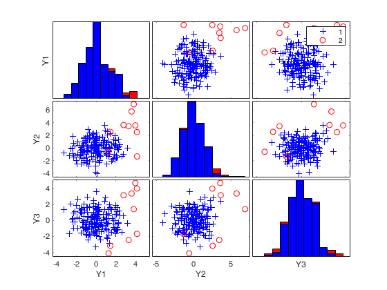
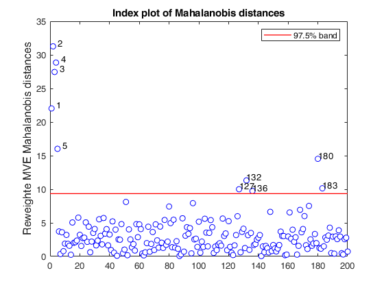
RAW=mve(Ycont,'plots',1);Warning: Using 'state' to set RANDN's internal state causes RAND, RANDI, and RANDN to use legacy random number generators. This syntax is not recommended. See <a href="matlab:helpview([docroot '\techdoc\math\math.map'],'update_random_number_generator')">Replace Discouraged Syntaxes of rand and randn</a> to use RNG to replace the old syntax. Total estimated time to complete MVE: 0.60 seconds


mve monitoring the extracted subsamples.
mve monitoring the extracted subsamples.
n=200;
v=3;
randn('state', 123456);
Y=randn(n,v);
% Contaminated data
Ycont=Y;
Ycont(1:5,:)=Ycont(1:5,:)+3;
[RAW,REW,C]=mve(Ycont);
Total estimated time to complete MVE: 0.52 seconds
Input Arguments
Output Arguments
More About
References
Rousseeuw, P.J. (1984), Least Median of Squares Regression, "Journal of the American Statistical Association", Vol. 79, pp. 871-881.
Rousseeuw, P.J. and Leroy A.M. (1987), Robust regression and outlier detection, Wiley New York.
Acknowledgements
This function follows the lines of MATLAB/R code developed during the years by many authors.
For more details see the R library robustbase http://robustbase.r-forge.r-project.org/ The core of these routines, e.g. the resampling approach, however, has been completely redesigned, with considerable increase of the computational performance.