qqplotFS
qqplotFS creates qqplot of studentized residuals with envelopes
Description
Displays a quantile-quantile plot of the quantiles of the sample studentized residuals versus the theoretical quantile values from a normal distribution. If the distribution of residuals is normal, then the data plot appears linear. A confidence level is added to the band.
qqplot with envelopes for the Wool data.Y
=qqplotFS(res,
Name, Value)
Examples
 qqplot for the multiple regression data.
qqplot for the multiple regression data.This is an example of the use of options X and plots
load('multiple_regression.txt');
y=multiple_regression(:,4);
X=multiple_regression(:,1:3);
outLM=fitlm(X,y,'exclude','');
res=outLM.Residuals{:,3};
qqplotFS(res,'X',X,'plots',1);
title('qqplot of stud. res.')
% No outlier appears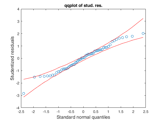
qqplot with envelopes for the Wool data.
qqplot with envelopes for the Wool data.Compare the results using untransformed and transformed data.
% This is an example of the use of option h
XX=load('wool.txt');
y=(XX(:,end));
lny=log(y);
X=XX(:,1:end-1);
outLM=fitlm(X,y,'exclude','');
res=outLM.Residuals{:,3};
outLMtra=fitlm(X,lny,'exclude','');
restra=outLMtra.Residuals{:,3};
h1=subplot(1,2,1);
qqplotFS(res,'X',X,'plots',1,'h',h1);
title('QQplot using untransformed data')
h2=subplot(1,2,2);
qqplotFS(restra,'X',X,'plots',1,'h',h2);
title('QQplot using transformed data')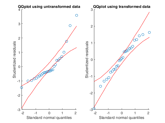

Input Arguments
Output Arguments
References
Atkinson, A.C. and Riani, M. (2000), "Robust Diagnostic Regression Analysis", Springer Verlag, New York.