Forward search in linear regression with exploratory data analysis (EDA) purposes

The Forward search in linear regression, used for exploratory data analysis (EDA) purposes, monitors the evolution of residuals, parameters estimates and inferences as the subset size increases. In other words, the results are presented as as “forward plots” which show the evolution of the quantities of interest as a function of the subset size. Therefore, unlike other robust approaches, the forward search is a dynamic process that produces a sequence of estimates and related plots. In this page, in order to compare the output of the forward plots with that based from the application of traditional robust estimators we concentrate our attention on the same dataset (loyalty cards) which had already been analyzed in page "Least trimmed squares (LTS) and Least median of squares (LMS)".

% Load the data
load('loyalty.txt');
nameX={'Intercept' 'Number of visits', 'Age', 'Number of persons in the family'};
% define y and X
y=loyalty(:,4);
X=loyalty(:,1:3);
% transform y
y1=y.^(0.4);
[out]=LXS(y1,X);
% Use function FSReda (Forward search in linear regression with EDA purposes) in order to store the relevant quantities.
[out]=FSReda(y1,X,out.bs);

In this page in order to illustrate the power of the forward plots to reveal the real structure of the data we give a series of forward plots

Monitoring residuals plot without labeling any trajectory can be obtained from the following code.

fground=struct;
fground.flabstep='';
resfwdplot(out,'fground',fground);

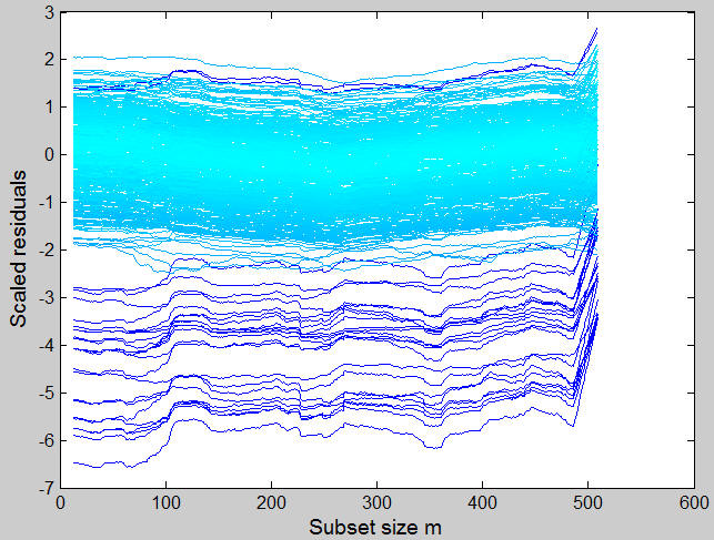
The monitoring residuals plot shows that there is a group of trajectories which have a very large negative residual throughout all the central part of the search and that at the end their trajectories are completely confused with those of the rest of the data.

Remark: it is interesting to notice the similarity of these trajectories during all steps the search: they tend to respond in the same way to the inclusion of units into the subset.

 

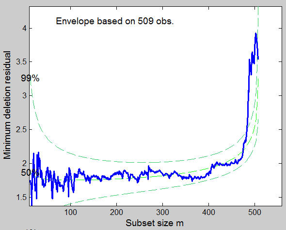
Another plot which helps to reveal the presence of atypical observations is the Monitoring of minimum deletion residual among observations not belonging to the subset. This plot clearly reveals that in the final part of the search there is a set of observations whose minimum deletion residual lies well above the 99% simulation envelope. It is interesting to notice that the final value of the statistic when $m = n -1$ lies inside the envelope, so that the outliers are masked.

mdrplot(out);

 

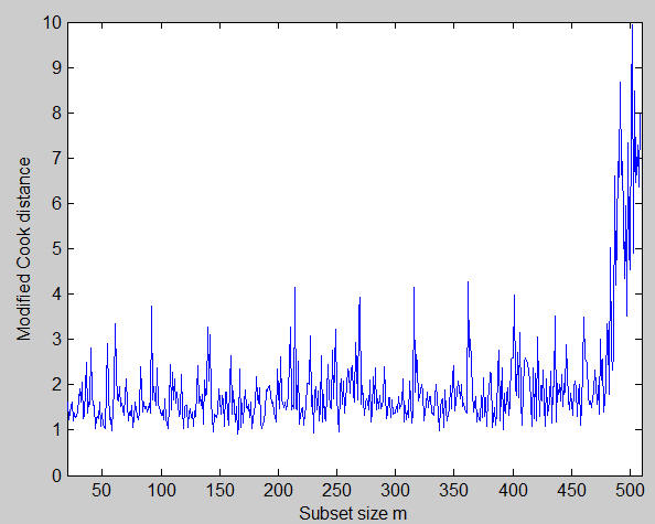
In order to understand the effect the last units which enter the search exert on the fitted model we also plot the Monitoring of modified Cook distance

plot(out.coo(:,1),out.coo(:,3))
ylabel('Modified Cook distance');
xlabel('Subset size m');
xlim([20 510])

This plot shows in the final part of the search, when the outliers enter the subset, a big sudden increase.

In order to understand what are the components of the estimated parameter vector  which are affected mostly by the introduction of the last units we can monitor in separate panels the estimates of the elements of the vector of beta. This plot can be produced efficiently using the loop which follows:

figure;
for j=2:size(out.Bols,2);
    subplot(2,2,j-1)
    plot(out.Bols(:,1),out.Bols(:,j))
    xlim([10 510])
    xlabel('Subset size m');
    ylabel(nameX(j-1));
end

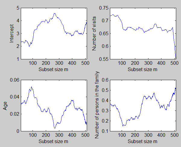
This plot shows that the effect of the outliers is mainly to decrease the estimated coefficient  linked to the "number of visits" to the supermarket.

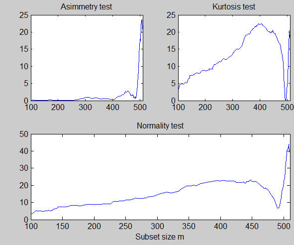
The monitoring residuals plot showed that the last observations which enter the search are characterized by negative residuals. The monitoring of the normality test, especially in the part associated to asymmetry, shows that the effect of the units which enter the final part of the search is to produce a distribution with a long left tail and to increase considerably the value of the normality test.

xlimx=[100 510];
subplot(2,2,1);
plot(out.nor(:,1),out.nor(:,2));
title('Asimmetry test');
xlim(xlimx);

subplot(2,2,2)
plot(out.nor(:,1),out.nor(:,3))
title('Kurtosis test');
xlim(xlimx);

subplot(2,2,3:4)
plot(out.nor(:,1),out.nor(:,4))
xlim(xlimx);
title('Normality test');
xlabel('Subset size m');