rthin
rthin applies independent random thinning to a point pattern.
Description
This function was ported to matlab from the R spatstat package, developed by Adrian Baddeley (Adrian.Baddeley@curtin.edu.au), Rolf Turner (r.turner@auckland.ac.nz) and Ege Rubak (rubak@math.aau.dk) for the statistical analysis of spatial point patterns. The algorithm for random thinning was changed in spatstat version 1.42-3. Our matlab porting is based on a earlier version. See the rthin documentation in spatstat for more details.
In a random thinning operation, each point of X is randomly either deleted or retained (i.e. not deleted). The result is a point pattern, consisting of those points of X that were retained. Independent random thinning means that the retention/deletion of each point is independent of other points.
Examples
 Random thinning on a mixture of normal distribution.
Random thinning on a mixture of normal distribution.Data
clear all; close all;
data=[randn(500,2);randn(500,1)+3.5, randn(500,1);];
x = data(:,1);
y = data(:,2);
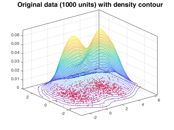
% Data density
[density,xout,bandwidth] = kdebiv(data,'pdfmethod','fsda');
xx = xout(:,1);
yy = xout(:,2);
zz = density;
% plot of data and density
figure;
[xq,yq] = meshgrid(xx,yy);
density = griddata(xx,yy,density,xq,yq);
contour3(xq,yq,density,50), hold on
plot(x,y,'r.','MarkerSize',5)
title(['Original data (' num2str(numel(y)) ' units) with density contour'],'FontSize',16);
%Interpolate the density and apply thinning using retention probabilities (1 - pdfe/max(pdfe))
F = TriScatteredInterp(xx(:),yy(:),zz(:));
pdfe = F(x,y);
pretain = 1 - pdfe/max(pdfe);
[Xt , Xti]= rthin([x y],pretain);
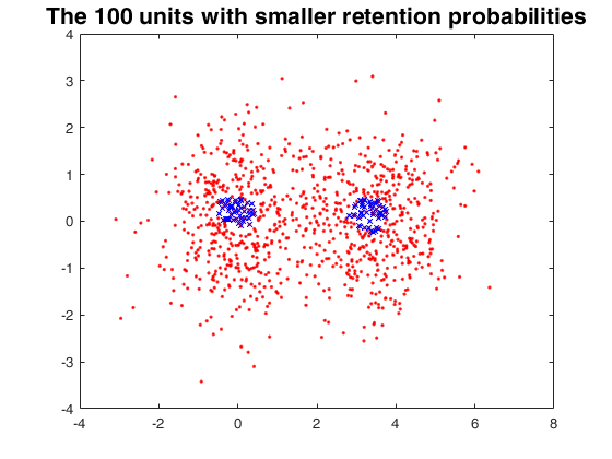
% rthin retention probabilities
[psorted ii] = sort(pretain);
figure;
plot(x,y,'r.','MarkerSize',5);
hold on;
plot(x(ii(1:100)),y(ii(1:100)),'bx','MarkerSize',5);
title('The 100 units with smaller retention probabilities','FontSize',16);
% now estimate the density on the retained units
%[tdensity,txout,tbandwidth] = ksdensity(Xt);
[tdensity,txout,tbandwidth] = kdebiv(Xt,'pdfmethod','fsda');
txx = txout(:,1);
tyy = txout(:,2);
tzz = tdensity;
% and plot the retained units with their density superimposed
figure;
[txq,tyq] = meshgrid(txx,tyy);
tdensity = griddata(txx,tyy,tdensity,txq,tyq);
contour3(txq,tyq,tdensity,50), hold on
plot(x(Xti),y(Xti),'b.','MarkerSize',5);
title(['Retained data (' num2str(numel(y(Xti))) ' units) with new density contour'],'FontSize',16);
cascade;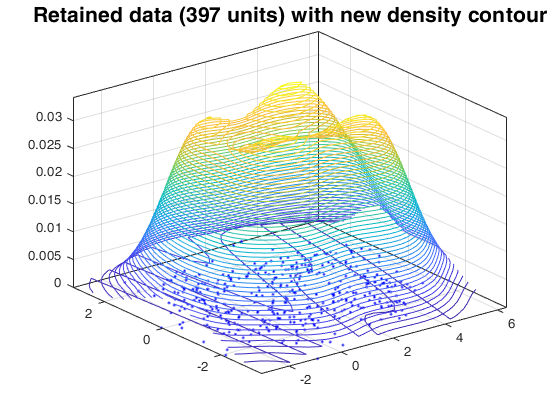
Random thinning on the fishery dataset.
Random thinning on the fishery dataset.load data and add some jittering, because duplicated units are not treated
clear all; close all;
load('fishery.txt');
fishery = fishery + 10^(-8) * abs(randn(677,2));
x = fishery(:,1);
y = fishery(:,2);
% Data density
[density,xout,bandwidth] = kdebiv(fishery,'pdfmethod','fsda');
xx = xout(:,1);
yy = xout(:,2);
zz = density;
% plot of data and density
figure;
[xq,yq] = meshgrid(xx,yy);
density = griddata(xx,yy,density,xq,yq);
contour3(xq,yq,density,50), hold on
plot(x,y,'r.','MarkerSize',8)
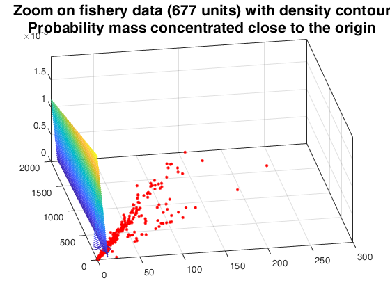
xlim([0 300]); ylim([0 2000]);
set(gca,'CameraPosition',[-216 -12425 0.0135]);
title({['Zoom on fishery data (' num2str(numel(y)) ' units) with density contour'] , 'Probability mass concentrated close to the origin'},'FontSize',16);
%Interpolate the density and apply thinning using retention
%probabilities equal to 1 - pdfe/max(pdfe)
F = TriScatteredInterp(xx(:),yy(:),zz(:));
pdfe = F(x,y);
pretain = 1 - pdfe/max(pdfe);
[Xt , Xti]= rthin([x y],pretain);
% now estimate the density on the retained units
[tdensity,txout,tbandwidth] = kdebiv(Xt,'pdfmethod','fsda');
txx = txout(:,1);
tyy = txout(:,2);
tzz = tdensity;
% and plot the retained units with their density superimposed
figure;
[txq,tyq] = meshgrid(txx,tyy);
tdensity = griddata(txx,tyy,tdensity,txq,tyq);
contour3(txq,tyq,tdensity,50), hold on
plot(x(Xti),y(Xti),'b.','MarkerSize',8);
xlim([0 300]); ylim([0 2000]);
set(gca,'CameraPosition',[-216 -12425 0.0002558 ]);
title({['Zoom on retained on the fishery data (' num2str(numel(y(Xti))) ' units) with density contour'] , 'Probabiity mass is smoother'},'FontSize',16);
cascade;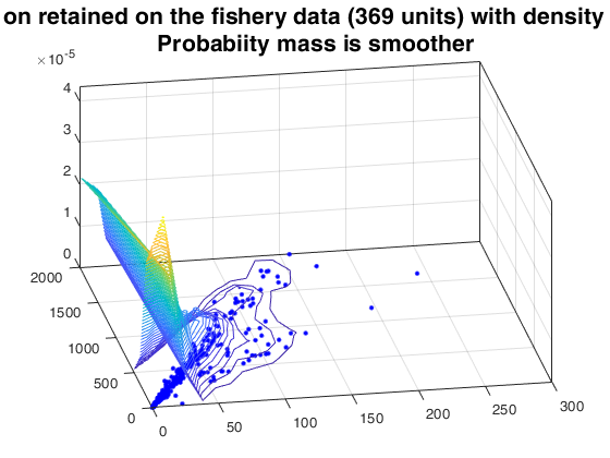
Input Arguments
Output Arguments
References
Bowman, A.W. and Azzalini, A. (1997), "Applied Smoothing Techniques for Data Analysis", Oxford University Press.
Acknowledgements
This function was ported to matlab from the R spatstat package, developed by Adrian Baddeley (Adrian.Baddeley@curtin.edu.au), Rolf Turner (r.turner@auckland.ac.nz) and Ege Rubak (rubak@math.aau.dk) for the statistical analysis of spatial point patterns. The algorithm for random thinning was changed in spatstat version 1.42-3. Our matlab porting is based on a previous version. See the rthin documentation in spatstat for more details.