simulateTS
simulateTS simulates a time series with trend, time varying seasonal, level shift and irregular component.
Description
simulateTS simulates a time series with trend (up to third order), seasonality (constant or of varying amplitude) with a different number of harmonics and a level shift. Moreover, it is possible to add to the series the effect of explanatory variables.
Same as above, but without homogenizing the y-scale.out
=simulateTS(T,
Name, Value)
Examples
 Simulated time series with linear trend.
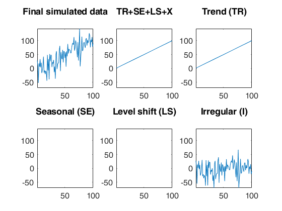
Simulated time series with linear trend.A time series of 100 observations is simulated from a model that contains a linear trend (with slope 1 and intercept 0), no seasonal component, no explanatory variables and a signal to noise ratio equal to 1 (the default).
out=simulateTS(100,'plots',1);
None of the inputs for simulating residuals has been specified. The default value signal2noiseratio=1 will be considered.
Related Examples
Simulated time series with a linear time varying seasonal component.
Simulated time series with a linear time varying seasonal component.A time series of 100 observations is simulated from a model that contains no trend, a linear time varying seasonal component with three harmonics, no explanatory variables and a signal to noise ratio equal to 20.
rng('default')
rng(1)
model=struct;
model.trend=[];
model.trendb=[];
model.seasonal=103;
model.seasonalb=40*[0.1 -0.5 0.2 -0.3 0.3 -0.1 0.222];
model.signal2noiseratio=20;
T=100;
out=simulateTS(T,'model',model,'plots',1);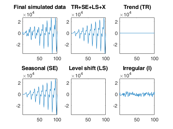
Simulated time series with a quadratic time varying seasonal component.
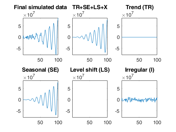
Simulated time series with a quadratic time varying seasonal component.A time series of 100 observations is simulated from a model that contains no trend, a quadratic time varying seasonal component with one harmonic, no explanatory variables and a signal to noise ratio equal to 20.
rng(1)
model=struct;
model.trend=[];
model.trendb=[];
model.seasonal=201;
model.seasonalb=40*[0.1 -0.5 10.222 -10];
model.signal2noiseratio=20;
T=100;
out=simulateTS(T,'model',model,'plots',1);
Simulated time series with quadratic trend, fixed seasonal and level shift.
Simulated time series with quadratic trend, fixed seasonal and level shift.A time series of 100 observations is simulated from a model that contains a quadratic trend, a seasonal component with two harmonics, no explanatory variables and a level shift in position 30 with size 5000 and a signal to noise ratio equal to 20.
rng(1)
model=struct;
model.trend=2;
model.trendb=[5,10,-3];
model.seasonal=2;
model.seasonalb=100*[2 4 0.1 8];
model.signal2noiseratio=20;
model.lshift=30;
model.lshiftb=5000;
T=100;
out=simulateTS(T,'model',model,'plots',1);
Simulated time series with quadratic trend, fixed seasonal and LS.
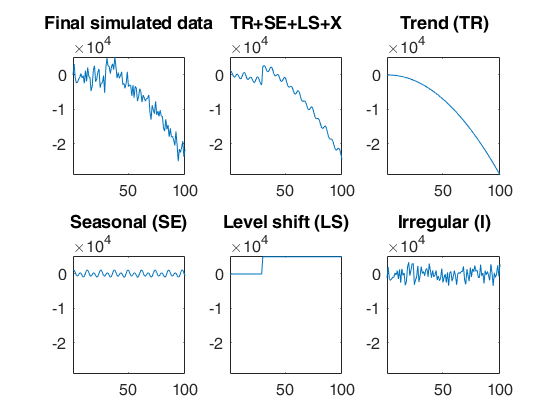
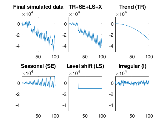
Simulated time series with quadratic trend, fixed seasonal and LS.A time series of 100 observations is simulated from a model that contains a quadratic trend, a linear time varying seasonal component with two harmonics, no explanatory variables and a level shift in position 30 with size -10000 and a signal to noise ratio equal to 20.
rng(1)
model=struct;
model.trend=2;
model.trendb=[5,10,-3];
model.seasonal=102;
model.seasonalb=100*[2 4 0.1 8 0.001];
model.signal2noiseratio=20;
model.lshift=30;
model.lshiftb=-10000;
T=100;
out=simulateTS(T,'model',model,'plots',1);
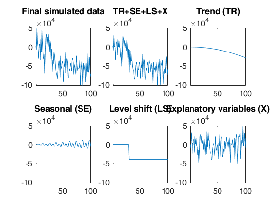
Simulated time series with quadratic trend, fixed seasonal, LS and two explanatory variables.
Simulated time series with quadratic trend, fixed seasonal, LS and two explanatory variables.A time series of 100 observations is simulated from a model that contains a quadratic trend, a linear time varying seasonal component with two harmonics, two explanatory variables and a level shift in position 30 with size -40000 and a signal to noise ratio equal to 10.
rng(1)
model=struct;
model.trend=2;
model.trendb=[5,10,-3];
model.seasonal=102;
model.seasonalb=100*[2 4 0.1 8 0.001];
model.signal2noiseratio=10;
model.lshift=30;
model.lshiftb=-40000;
model.X=2;
model.Xb=[10000 20000];
T=100;
out=simulateTS(T,'model',model,'plots',1);
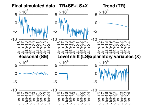
Example of the use of option StartDate.
Example of the use of option StartDate.Suppose that the initial observation refers to February 2016.
StartDate=[2016 2];
% The x axis of the plots contains the dates using format mmm-yy.
rng(1)
model=struct;
model.trend=2;
model.trendb=[5,10,-3];
model.seasonal=102;
model.seasonalb=100*[2 4 0.1 8 0.001];
model.signal2noiseratio=10;
model.lshift=30;
model.lshiftb=-40000;
model.X=2;
model.Xb=[10000 20000];
T=100;
out=simulateTS(T,'model',model,'plots',1,'StartDate',StartDate);
Input Arguments
Output Arguments
References
Rousseeuw, P.J., Perrotta D., Riani M. and Hubert, M. (2018), Robust Monitoring of Many Time Series with Application to Fraud Detection, "Econometrics and Statistics". [RPRH]