twdpdf
twdpdf computes the probability density function of the Tweedie distribution.
Syntax
pdf=twdpdf(x,alpha,theta,delta)example
Description
Examples
Related Examples
 Check consistency with R theedie package.
Check consistency with R theedie package.Note that the package adopts the parametrization of Jorgensen (1987), which introduces the Tweedie distribution as a special case of the exponential dispersion model.
% In the R tweedie package, the parameters are:
% p     = vector of probabilities;
% n     = the number of observations;
% xi    = the value of xi such that the variance is $var(Y)=\phi \mu^{xi}$;
% power = a synonym for xi
% mu    = the mean
% phi	= the dispersion
% # R code
% power <- 2.5
% mu    <- 1
% phi   <- 1
% y     <- seq(0, 6, length=500)
% fy    <- dtweedie( y=y, power=power, mu=mu, phi=phi)
% plot(y, fy, type="l", lwd=2, ylab="Density")
% # Compare to the saddlepoint density
% f.saddle <- dtweedie.saddle( y=y, power=power, mu=mu, phi=phi)
% lines( y, f.saddle, col=2 )
% legend("topright", col=c(1,2), lwd=c(2,1),
%     legend=c("Actual","Saddlepoint") )
% parameter values in Jorgensen parametrization
power = 2.5;
mu    = 1 ;
phi   = 1 ;
% reparametrization
alpha = (power-2)/(power-1);
theta = phi*mu;
delta = (phi/(power-1))^(1/(power-1));
% pdf
y = linspace(0,6,500);
pdf = twdpdf(y,alpha,theta,delta);
figure;
subplot(2,1,1);
plot(y,pdf,'r.');
title({'Jorgensen parametrization: power = 2.5, mu = 1, phi = 1' , ...
're-parametrization: alpha = 0.3333, theta = 1, delta = 0.7631'});
Y = twdrnd(alpha,theta,delta,500);
subplot(2,1,2);
histogram(Y);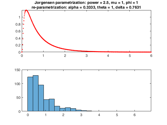
Input Arguments
Output Arguments
More About
References
Tweedie, M. C. K. (1984), An index which distinguishes between some important exponential families, "in Statistics: Applications and New Directions, Proceedings of the Indian Statistical Institute Golden Jubilee International Conference (J.K. Ghosh and J. Roy, eds.), Indian Statistical Institute, Calcutta", pp. 579-604.