unibiv
unibiv has the purpose of detecting univariate and bivariate outliers
Description
Examples
unibiv with all default options.
Run this code to see the output shown in the help file
n=500;
p=5;
randn('state', 123456);
Y=randn(n,p);
[out]=unibiv(Y);
 unibiv with optional arguments.
unibiv with optional arguments.Stack loss data.
Y=load('stack_loss.txt');
% Show robust confidence ellipses
out=unibiv(Y,'plots',1,'textlab',1);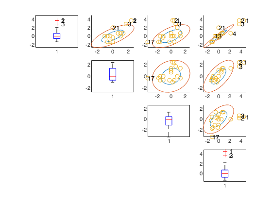
Input Arguments
Y — Input data.
Matrix.
n x v data matrix; n observations and v variables. Rows of Y represent observations, and columns represent variables.
Missing values (NaN's) and infinite values (Inf's) are allowed, since observations (rows) with missing or infinite values will automatically be excluded from the computations.
Data Types: single|double
Name-Value Pair Arguments
Specify optional comma-separated pairs of Name,Value arguments.
Name is the argument name and Value
is the corresponding value. Name must appear
inside single quotes (' ').
You can specify several name and value pair arguments in any order as
Name1,Value1,...,NameN,ValueN.
 'madcoef',2
, 'rf',0.99
, 'robscale',2
, 'plots',2
, 'tag','new_tag'
, 'textlab',0
madcoef
—scaled MAD.scalar.
Coefficient which is used to scale MAD coefficient to have a robust estimate of dispersion. The default is 1.4815 so that 1.4815*MAD(N(0,1))=1.
Remark: if mad =median(y-median(y))=0 then the interquartile range is used. If also the interquartile range is 0 than the MD (mean absolute deviation) is used. In other words MD=mean(abs(y-mean(Y))
Example: 'madcoef',2
Data Types: double
rf
—It specifies the confidence
level of the robust bivariate ellipses.scalar.
0<rf<1.
The default value is 0.95 that is the outer contour in presence of normality for each ellipse should leave outside 5% of the values.
Example: 'rf',0.99
Data Types: double
robscale
—how to compute dispersion.scalar.
It specifies the statistical indexes to use to compute the dispersion of each variable and the correlation among each pair of variables.
robscale=1 (default): the program uses the median correlation and the MAD as estimate of the dispersion of each variable;
robscale=2: the correlation coefficient among ranks is used (Spearman's rho) and the MAD as estimate of the dispersion of each variable;
robscale=3: the correlation coefficient is based on Kendall's tau b and the MAD as estimate of the dispersion of each variable;
robscale=4: tetracoric correlation coefficient is used and the MAD as estimate of the dispersion of each variable;
otherwise the correlation and the dispersion of the variables are computed using the traditional (non robust) formulae around the univariate medians.
Example: 'robscale',2
Data Types: double
plots
—Plot on the screen.scalar.
It specifies whether it is necessary to produce a plot with univariate standardized boxplots on the main diagonal and bivariate confidence ellipses out of the main diagonal. If plots is equal to 1 a plot which contains univariate standardized boxplots on the main diagonal and bivariate confidence ellipses out of the main diagonal is produced on the screen. If plots is <> 1 no plot is produced. As default no plot is produced.
Example: 'plots',2
Data Types: double
tag
—plot tag.character.
It identifies the handle of the plot which is about to be created. The default is to use tag 'pl_unibiv'. Notice that if the program finds a plot which has a tag equal to the one specified by the user, then the output of the new plot overwrites the existing one in the same window else a new window is created.
Example: 'tag','new_tag'
Data Types: char
textlab
—plot labels.scalar.
Scalar which controls the labels in the plots. If textlab=1 and plots=1 the labels associated to the units which are univariate outliers or which are outside the confidence levels of the contours are displayed on the screen.
Example: 'textlab',0
Data Types: double
Output Arguments
fre —Details about the univariate and
bivariate outliers.
n -by- 4 matrix
1st col = index of the units;
2nd col = number of times unit has been declared univariate outliers;
3rd col = number of times unit has been declared bivariate outlier;
4th col = pseudo MD as sum of bivariate MD.
References
Riani, M., Zani S. (1997). An iterative method for the detection of multivariate outliers, "Metron", Vol. LV, pp. 101-117.