wthin

wthin thins a uni/bi-dimensional dataset

Syntax

Description

Computes retention probabilities and bernoulli (0/1) weights on the basis of data density estimate.

example

Wt =wthin(X) Univariate thinning.

example

Wt =wthin(X, Name, Value) Bi-dimensional thinning.

example

[Wt, pretain] =wthin(___) Use of 'retainby' option.

example

[Wt, pretain, varargout] =wthin(___) Optional output Xt.

Examples

expand all

  • Univariate thinning.
  • clear all; close all;
    % The dataset is bi-dimensional and contain two collinear groups with
    % regression structure. One group is dense, with 1000 units; the second
    % has 100 units. Thinning in done according to the density of the values
    % predicted by the OLS fit.
    x1 = randn(1000,1);
    x2 = 8 + randn(100,1);
    x = [x1 ; x2];
    y = 5*x + 0.9*randn(1100,1);
    b = [ones(1100,1) , x] \ y;
    yhat = [ones(1100,1) , x] * b;
    plot(x,y,'.',x,yhat);
    %x3 = 0.2 + 0.01*randn(1000,1);
    %y3 = 40 + 0.01*randn(1000,1);
    %plot(x,y,'.',x,yhat,'--',x3,y3,'.');
    % thinning over the predicted values
    %[Wt,pretain] = wthin([yhat ; y3], 'retainby','comp2one');
    % thinning over the predicted values when specifying a thinning
    %probability pstar (randomized thinning).
    pstar=0.95
    [Wt,pretain] = wthin(yhat, 'retainby','comp2one','pstar',pstar);
    % thinning over the predicted values when specifying a thinning
    %cup (winsorized thinning).
    cup=0.5
    [Wt,pretain] = wthin(yhat, 'retainby','comp2one','cup',cup);
    figure;
    plot(x(Wt,:),y(Wt,:),'k.',x(~Wt,:),y(~Wt,:),'r.');
    drawnow;
    axis manual;
    title('univariate thinning over predicted ols values')
    clickableMultiLegend(['Retained: ' num2str(sum(Wt))],['Thinned:   ' num2str(sum(~Wt))]);

  • Bi-dimensional thinning.
  • Same dataset, but thinning is done on the original bi-variate data.

    x1 = randn(1000,1);
    x2 = 8 + randn(100,1);
    x = [x1 ; x2];
    y = 5*x + 0.9*randn(1100,1);
    b = [ones(1100,1) , x] \ y;
    plot(x,y,'.');
    % thinning over the original bi-variate data
    [Wt2,pretain2] = wthin([x,y]);
    plot(x(Wt2,:),y(Wt2,:),'k.',x(~Wt2,:),y(~Wt2,:),'r.');
    drawnow;
    axis manual;
    title('bivariate thinning')
    clickableMultiLegend(['Retained: ' num2str(sum(Wt2))],['Thinned:   ' num2str(sum(~Wt2))]);

  • Use of 'retainby' option.
  • Since the thinning on the original bi-variate data with the default retention method ('inverse') removes too many units, let's try with the less conservative 'comp2one' option.

    x1 = randn(1000,1);
    x2 = 8 + randn(100,1);
    x = [x1 ; x2];
    y = 5*x + 0.9*randn(1100,1);
    b = [ones(1100,1) , x] \ y;
    plot(x,y,'.');
    % thinning over the original bi-variate data
    [Wt2,pretain2] = wthin([x,y], 'retainby','comp2one');
    plot(x(Wt2,:),y(Wt2,:),'k.',x(~Wt2,:),y(~Wt2,:),'r.');
    drawnow;
    axis manual
    clickableMultiLegend(['Retained: ' num2str(sum(Wt2))],['Thinned:   ' num2str(sum(~Wt2))]);
    title('"comp2one" thinning over the original bi-variate data');

  • Optional output Xt.
  • Same dataset, the retained data are also returned using varagout option.

    x1 = randn(1000,1);
    x2 = 8 + randn(100,1);
    x = [x1 ; x2];
    y = 5*x + 0.9*randn(1100,1);
    % thinning over the original bi-variate data
    [Wt2,pretain2,RetUnits] = wthin([x,y]);
    % disp(RetUnits)

    Related Examples

    expand all

  • thinning on the fishery dataset.
  • load fishery;
    X=fishery{:,:};
    % some jittering is necessary because duplicated units are not treated
    % in tclustreg: this needs to be addressed
    X = X + 10^(-8) * abs(randn(677,2));
    % thinning over the original bi-variate data
    [Wt3,pretain3,RetUnits3] = wthin(X ,'retainby','comp2one');
    figure;
    plot(X(Wt3,1),X(Wt3,2),'k.',X(~Wt3,1),X(~Wt3,2),'rx');
    drawnow;
    axis manual
    clickableMultiLegend(['Retained: ' num2str(sum(Wt3))],['Thinned:   ' num2str(sum(~Wt3))]);
    title('"comp2one" thinning on the fishery dataset');

  • thinning on the fishery dataset using 'positive' support.
  • load fishery;
    X=fishery{:,:};
    % some jittering is necessary because duplicated units are not treated
    % in tclustreg: this needs to be addressed
    X = X + 10^(-8) * abs(randn(677,2));
    % thinning over the original bi-variate data
    [Wt3,pretain3,RetUnits3] = wthin(X ,'retainby','comp2one','support','positive');
    figure;
    plot(X(Wt3,1),X(Wt3,2),'k.',X(~Wt3,1),X(~Wt3,2),'rx');
    drawnow;
    axis manual
    clickableMultiLegend(['Retained: ' num2str(sum(Wt3))],['Thinned:   ' num2str(sum(~Wt3))]);
    title('"comp2one" thinning on the fishery dataset, using positive support');
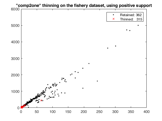
    Click here for the graphical output of this example (link to Ro.S.A. website)

  • univariate thinning with less than 100 units.
  • As the first examp[le above, but with less than 100 units in the data.

    x1 = randn(850,1);
    x2 = 8 + randn(10,1);
    x = [x1 ; x2];
    y = 5*x + 0.9*randn(860,1);
    b = [ones(860,1) , x] \ y;
    yhat = [ones(860,1) , x] * b;
    plot(x,y,'.',x,yhat,'--');
    % thinning over the predicted values
    [Wt,pretain] = wthin(yhat, 'retainby','comp2one');
    plot(x(Wt,:),y(Wt,:),'k.',x(~Wt,:),y(~Wt,:),'r.');
    drawnow;
    axis manual
    title('univariate thinning over ols values predicted on a small dataset')
    clickableMultiLegend(['Retained: ' num2str(sum(Wt))],['Thinned:   ' num2str(sum(~Wt))]);

    Input Arguments

    expand all

    X — Input data. Vector or 2-column matrix.

    The structure contains the uni/bi-variate data to be thinned on the basis of a probability density estimate.

    Data Types: single| double

    Name-Value Pair Arguments

    Specify optional comma-separated pairs of Name,Value arguments. Name is the argument name and Value is the corresponding value. Name must appear inside single quotes (' '). You can specify several name and value pair arguments in any order as Name1,Value1,...,NameN,ValueN.

    Example: bandwidth,0.35 , support,'positive' , cup, 0.8 , pstar, 0.95 , 'method','comp2one'

    bandwidth —bandwidth value.scalar.

    The bandwidth used to estimate the density. It can be estimated from the data using function bwe.

    Example: bandwidth,0.35

    Data Types: scalar

    support —support value.character array.

    The support of the density estimation step. It can be 'unbounded' (the default) or 'positive' if the data are left-truncated with long right tails. In the latter case, the option performs the density estimate in the log domain and then transform the result back. The theoretical rationale is that when kernel density is applied to positive data, it does not yield proper PDFs.

    Example: support,'positive'

    Data Types: char

    cup —pdf upper limit.scalar.

    The upper limit for the pdf used to compute the retantion probability. If cup = 1 (default), no upper limit is set.

    Example: cup, 0.8

    Data Types: scalar

    pstar —thinning probability.scalar.

    Probability with each a unit enters in the thinning procedure. If pstar = 1 (default), all units enter in the thinning procedure.

    Example: pstar, 0.95

    Data Types: scalar

    retainby —retention method.string.

    The function used to retain the observations. It can be: - 'inverse' , i.e. (1 ./ pdfe) / max((1 ./ pdfe))) - 'comp2one' (default), i.e. 1 - pdfe/max(pdfe))

    Example: 'method','comp2one'

    Data Types: char

    Output Arguments

    expand all

    Wt —vector of Bernoulli weights. Vector

    Contains 1 for retained units and 0 for thinned units.

    Data Types - single | double.

    pretain —vector of retention probabilities. Vector

    These are the probabilities that each point in X will be retained, estimated using a gaussian kernel using function ksdensity.

    Data Types - single | double.

    varargout —Xt : vector of retained units. Vector

    It is X(Wt,:).

    Data Types - single | double.

    References

    Bowman, A.W. and Azzalini, A. (1997), "Applied Smoothing Techniques for Data Analysis", Oxford University Press.

    Wand, M.P. and Marron, J.S. and Ruppert, D. (1991), "Transformations in density estimation", Journal of the American Statistical Association, 86(414), 343-353.

    This page has been automatically generated by our routine publishFS