mdEM
mdEM EM algorithm for data with missing values (no trimming)
Description
Examples
 Example of use of option condmeanimp.
Example of use of option condmeanimp.. number of variables
p = 15;
% number of observations
n = 1000;
% target pairwise correlation (0<rho<1)
rho = 0.9;
% Covariance matrix (unit variances)
Sigma = (1-rho)*eye(p) + rho*ones(p);
R = chol(Sigma);      % upper-triangular such that Sigma = R'*R
% Generate samples ~ N(0,Sigma)
Yfull = randn(n,p) * R;   % Strong positive correlation between the vars
missRate = 0.25;     % MCAR missing probability per entry
missMask = rand(n,p) < missRate;
Y=Yfull;
Y(missMask) = NaN;
% md with missing imputation
out=mdEM(Y,'condmeanimp',true);
% Mahalanobis distances using original matrix
d2Ori=mahalFS(Yfull,mean(Yfull),cov(Yfull));
% Calculate the Mahalanobis distance for the imputed data
d2Imp = mahalFS(out.Yimp, mean(out.Yimp), cov(out.Yimp));
% Compare original with distances for the imputed data
% Calculate the differences between original and imputed Mahalanobis distances
scatter(d2Ori,d2Imp)
% Add axis labels
xlabel('Original Mahalanobis Distances');
ylabel('Imputed Mahalanobis Distances');
grid on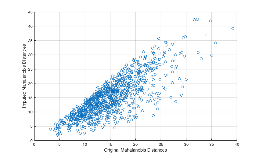
Related Examples
Example of use of option stochimp.
Example of use of option stochimp.number of variables
p = 15;
    % number of observations
    n = 1000;
    % target pairwise correlation (0<rho<1)
    rho = 0.9;
    % Covariance matrix (unit variances)
    Sigma = (1-rho)*eye(p) + rho*ones(p);
    R = chol(Sigma);      % upper-triangular such that Sigma = R'*R
    % Generate samples ~ N(0,Sigma)
    Yfull = randn(n,p) * R;   % Strong positive correlation between the vars
    missRate = 0.25;     % MCAR missing probability per entry
    missMask = rand(n,p) < missRate;
    Y=Yfull;
    Y(missMask) = NaN;
    % md with missing imputation
    out=mdEM(Y,'stochimp',true);
    % Mahalanobis distances using original matrix
    d2Ori=mahalFS(Yfull,mean(Yfull),cov(Yfull));
    % Calculate the Mahalanobis distance for the imputed data
    d2Imp = mahalFS(out.stochYimp, mean(out.stochYimp), cov(out.stochYimp));
    % Compare original with distances for the imputed data
    % Calculate the differences between original and imputed Mahalanobis distances
    scatter(d2Ori,d2Imp)
    % Add axis labels
    xlabel('Original Mahalanobis Distances');
    ylabel('Imputed Mahalanobis Distances (stochastic imputation)');
    grid on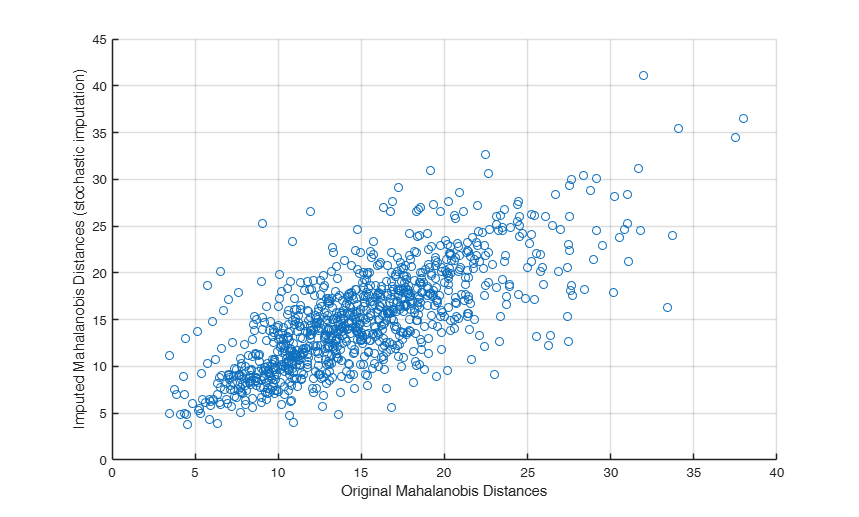
Example of use of options Patterns and idxPatterns.
Example of use of options Patterns and idxPatterns.number of variables
p = 3;
    % number of observations
    n = 50000;
    % target pairwise correlation (0<rho<1)
    rho = 0.9;
    % Covariance matrix (unit variances)
    Sigma = (1-rho)*eye(p) + rho*ones(p);
    R = chol(Sigma);      % upper-triangular such that Sigma = R'*R
    % Generate samples ~ N(0,Sigma)
    Yfull = randn(n,p) * R;   % Strong positive correlation between the vars
    missRate = 0.25;     % MCAR missing probability per entry
    missMask = rand(n,p) < missRate;
    Y=Yfull;
    Y(missMask) = NaN;
    M=ismissing(Y);
    [Patterns, ~, idxPatterns] = unique(M, 'rows', 'stable');
    disp('Computational time using missing patterns')
    tic
    outWITHPAT=mdEM(Y,'Patterns',Patterns,'idxPatterns',idxPatterns);
    toc
    disp('Computational time neglecting missing patterns')
    tic
    outNOPAT=mdEM(Y);
    toc
Computational time using missing patterns Elapsed time is 0.077916 seconds. Computational time neglecting missing patterns Elapsed time is 2.477940 seconds.
Input Arguments
Output Arguments
References
Little, R. J. A., & Rubin, D. B. (2019). Statistical Analysis with Missing Data (3rd ed.). Hoboken, NJ: John Wiley & Sons.
Templ, M. (2023). Visualization and Imputation of Missing Values: With Applications in R. Cham, Switzerland: Springer Nature.
See Also
mdTEM
|
mdImputeCondMean
|
mdImputeStochastic
|
mdPartialMD
|
mdPartialMD2full