mdTEM

mdTEM EM algorithm with trimming (TEM) for data with missing values

Syntax

Description

The algorithm:

- At each iteration compute adjusted partial Mahalanobis distances;

- Rank them and set weights w_i = 1 for the lowest n*(1-alpha) rows, else 0;

- Run E-step and M-step using these weights;

- Apply a consistency correction for the truncation induced by trimming (see input option consistencyfactor);

- Repeat until convergence or maxiter.

example

out =mdTEM(Y) Call to mdTEM with all the default options.

example

out =mdTEM(Y, Name, Value) Example of use of option condmeanimp.

Examples

expand all

  • Call to mdTEM with all the default options.
  • . True model (choose something correlated)

    p=5; n=200;
    A = randn(p);
    SigmaTrue = A'*A;
    D = diag(1 ./ sqrt(diag(SigmaTrue)));
    SigmaTrue = D * SigmaTrue * D;      % "correlation-like"
    muTrue = linspace(-1,1,p)';
    %  generate complete data
    Yfull = mvnrnd(muTrue', SigmaTrue, n);             % n x p
    missRate = 0.25;     % MCAR missing probability per entry
    missMask = rand(n,p) < missRate;
    Y=Yfull;
    Y(missMask) = NaN;
    out=mdTEM(Y);
    % Show true means and inputed means
    scatter(out.loc,muTrue)
    refline(1)
    xlabel('Imputed means')
    ylabel('True means')

  • Example of use of option condmeanimp.
  • . number of variables

    p = 15;
    % number of observations
    n = 1000;
    % target pairwise correlation (0<rho<1)
    rho = 0.9;
    % Covariance matrix (unit variances)
    Sigma = (1-rho)*eye(p) + rho*ones(p);
    R = chol(Sigma);      % upper-triangular such that Sigma = R'*R
    % Generate samples ~ N(0,Sigma)
    Yfull = randn(n,p) * R;   % Strong positive correlation between the vars
    missRate = 0.25;     % MCAR missing probability per entry
    missMask = rand(n,p) < missRate;
    Y=Yfull;
    Y(missMask) = NaN;
    % md with missing imputation
    out=mdTEM(Y,'condmeanimp',true);
    % Mahalanobis distances using original matrix
    d2Ori=mahalFS(Yfull,mean(Yfull),cov(Yfull));
    % Calculate the Mahalanobis distance for the imputed data
    d2Imp = mahalFS(out.Yimp, mean(out.Yimp), cov(out.Yimp));
    % Compare original with distances for the imputed data
    scatter(d2Ori,d2Imp)
    xlabel('Original Mahalanobis Distances');
    ylabel('Imputed Mahalanobis Distances');
    grid on
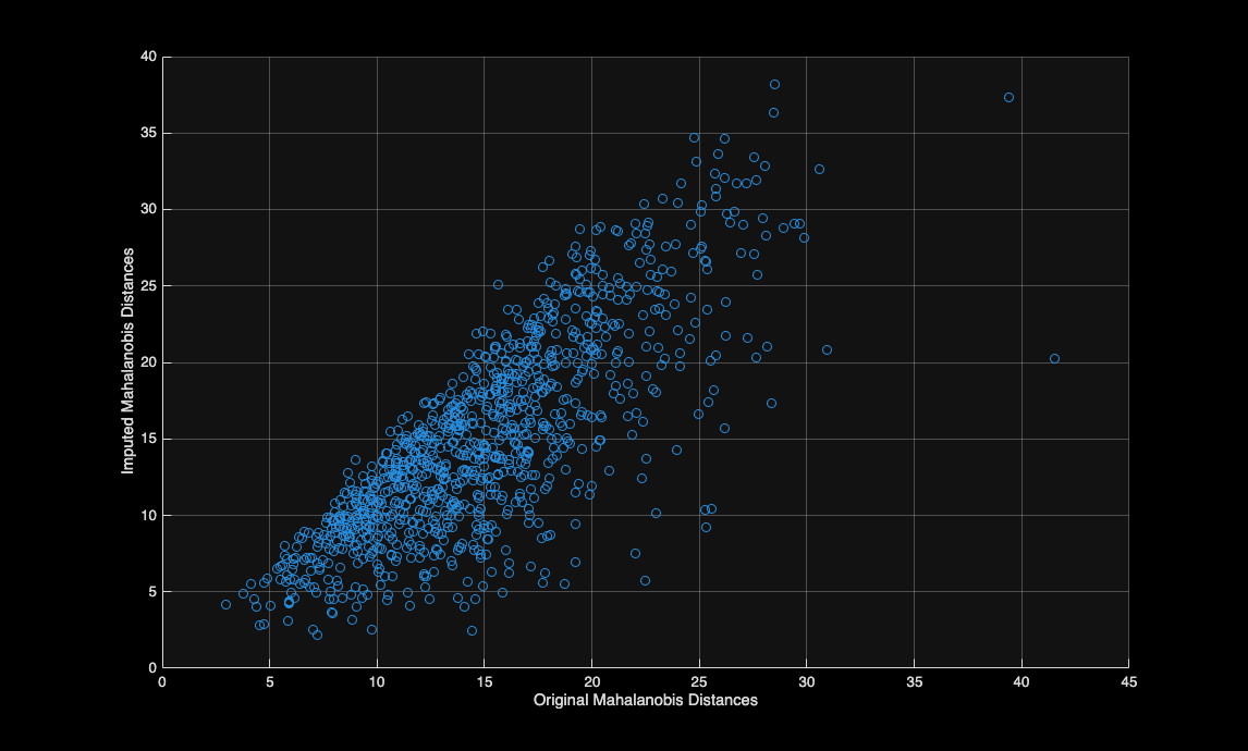
    Click here for the graphical output of this example (link to Ro.S.A. website).

    Related Examples

    expand all

  • Exact pattern-wise consistency correction.
  • The single global factor is exact only for the complete rows. The pattern-wise correction uses the exact factor for every missingness pattern and removes most of the residual downward bias of the scatter estimate.

    rng(7)
        p = 5;  n = 2000;  rho = 0.5;
        SigmaTrue = (1-rho)*eye(p) + rho*ones(p);
        Yfull = randn(n,p)*chol(SigmaTrue);
        Y = Yfull;
        Y(rand(n,p) < 0.35) = NaN;
        % rows left with no observed entry are put back
        allmiss = all(isnan(Y),2);
        Y(allmiss,1) = Yfull(allmiss,1);
    
        outG = mdTEM(Y,'alpha',0.5,'consistencyfactor','global');
        outP = mdTEM(Y,'alpha',0.5,'consistencyfactor','pattern');
    
        errG = max(max(abs(outG.cov-SigmaTrue)));
        errP = max(max(abs(outP.cov-SigmaTrue)));
        disp(['max |Sigma-hat - Sigma|, global  factor : ' num2str(errG)])
        disp(['max |Sigma-hat - Sigma|, pattern factors: ' num2str(errP)])
        % pattern-wise quantities of the last iteration
        disp(outP.kinfo)
    max |Sigma-hat - Sigma|, global  factor : 0.36913
    max |Sigma-hat - Sigma|, pattern factors: 0.24718
        pobs    nkept     athr      gammag       kg   
        ____    _____    _______    _______    _______
    
         5       94       4.4026    0.50698    0.52781
         4       65       3.4026    0.50716    0.47938
         4       68       3.4026    0.50716    0.47938
         3       35       2.4026    0.50685    0.41218
         4       59       3.4026    0.50716    0.47938
         3       29       2.4026    0.50685    0.41218
         3       28       2.4026    0.50685    0.41218
         2       18       1.4026    0.50407       0.31
         4       70       3.4026    0.50716    0.47938
         3       30       2.4026    0.50685    0.41218
         3       34       2.4026    0.50685    0.41218
         2       15       1.4026    0.50407       0.31
         3       35       2.4026    0.50685    0.41218
         2       22       1.4026    0.50407       0.31
         2       31       1.4026    0.50407       0.31
         1       17      0.40263    0.47427    0.12715
         4       57       3.4026    0.50716    0.47938
         3       37       2.4026    0.50685    0.41218
         3       34       2.4026    0.50685    0.41218
         2       18       1.4026    0.50407       0.31
         3       34       2.4026    0.50685    0.41218
         2       21       1.4026    0.50407       0.31
         2       23       1.4026    0.50407       0.31
         1       10      0.40263    0.47427    0.12715
         3       33       2.4026    0.50685    0.41218
         2       22       1.4026    0.50407       0.31
         2       20       1.4026    0.50407       0.31
         1        9      0.40263    0.47427    0.12715
         2        8       1.4026    0.50407       0.31
         1       15      0.40263    0.47427    0.12715
         1        9      0.40263    0.47427    0.12715


  • Diagnostic: are incomplete rows retained at the right rate? Under the null the share of incomplete rows in the retained subset should match their share in the whole sample.
  • rng(1)
        p = 7;  n = 10000;
        Y = randn(n,p);
        Y(rand(n,p) < 0.30) = NaN;
        allmiss = all(isnan(Y),2);  Y(allmiss,1) = randn(sum(allmiss),1);
        incomplete = any(isnan(Y),2);
        for cf = ["global" "pattern"]
            o = mdTEM(Y,'alpha',0.5,'consistencyfactor',cf);
            fprintf('%-8s share incomplete kept %.3f  (sample %.3f)\n', ...
                cf, mean(incomplete(o.weights==1)), mean(incomplete));
        end

    Input Arguments

    expand all

    Y — Input data. Matrix.

    n x p data matrix; n observations and v variables possibly with missing values (NaN's). Rows of Y represent observations, and columns represent variables.

    Data Types: single | double

    Name-Value Pair Arguments

    Specify optional comma-separated pairs of Name,Value arguments. Name is the argument name and Value is the corresponding value. Name must appear inside single quotes (' '). You can specify several name and value pair arguments in any order as Name1,Value1,...,NameN,ValueN.

    Example: 'alpha',0.1 , 'mus',[] , 'sigs',eye(p) , 'maxiter',50 , 'tol',1e-10 , 'tol_sigma',false , 'method','chiMap' , 'consistencyfactor','pattern' , 'condmeanimp',true , 'stochimp',true , 'storeobj',false

    alpha —proportion to trim.real number in the interval [0 0.

    5] or empty value.

    At each iteration compute adjusted partial Mahalanobis distance and set weights w_i = 1 for the lowest n*(1-alpha) rows. (e.g., 0.5 -> keep 50% with smallest distances). If alpha is empty the default value which is used is 0.5.

    Example: 'alpha',0.1

    Data Types: single | double

    mus —initial mean.p x 1 vector | empty double.

    Initial mean vector. If empty (default), column nanmeans are used.

    Example: 'mus',[]

    Data Types: single | double

    sigs —initial covariance matrix.p x p matrix | empty double.

    Initial p x p covariance matrix.

    If empty, uses nan-cov

    Example: 'sigs',eye(p)

    Data Types: single | double

    maxiter —maximum number of iterations.positive integer.

    The default value is 100

    Example: 'maxiter',50

    Data Types: single | double

    tol —tolerance for convergence.positive real number.

    The default value of the tolerance is 1e-5

    Example: 'tol',1e-10

    Data Types: single | double

    tol_sigma —Use tolerance for both mu sigs.boolean .

    If true use both mu and sigma diffs (default true)

    Example: 'tol_sigma',false

    Data Types: logical

    method —method used to rescale the distances.string scalar | char vector.

    Possible values are.

    'pri' = principled EM rescaling (default), d2_partial + (p - pobs).

    'expScale' = expectation scaling, d2_partial * (p / pobs).

    'zMap' = standardization mapping, p + sqrt(2*p) * ((d2_partial - pobs) ./ sqrt(2*pobs)).

    'detMap' = determinant-based rescaling, d2_partial * (p / pobs) * (g_full / g_obs).

    'chiMap' = chi-square quantile mapping. Use the cdf and inverse of the cdf of Chi2 distribution.

    'betaMap' = Beta quantile mapping. Use the cdf and inverse of the cdf of Beta distribution.

    'impMD' = MD on EM-imputed data.

    Example: 'method','chiMap'

    Data Types: string scalar | char vector

    consistencyfactor —treatment of the truncation bias of the scatter estimate.character vector | string scalar.

    Possible values:

    'global' = (default) single scalar factor k = (n/h)*F_{chi2_{p+2}}(a), a = chi2inv(h/n,p), applied to the whole scatter matrix. This is the complete-data Tallis factor evaluated at the full dimension p and at the global retained fraction h/n. It is exact only for the rows without missing entries.

    'pattern' = exact pattern-wise correction. Trimming on any strictly increasing adjustment induces, within each missingness pattern g, an exact radial truncation of the corresponding Gaussian marginal at the threshold a_g = phi_{p_g}^{-1}(c), where c is the h-th smallest adjusted distance and phi is the adjustment. Tallis's theorem then applies exactly with dimension p_g, giving gamma_g = F_{chi2_{p_g}}(a_g), k_g = F_{chi2_{p_g+2}}(a_g)/gamma_g.

    The correction is applied to the data-driven part of the expected second moment only; the conditional-variance term Sigma_{m|o} is a model-based quantity and is left uncorrected.

    The location estimate needs no correction.

    'weighted' = single scalar, but computed as the information-weighted average of the exact pattern-wise factors, kbar = sum_g h_g p_g k_g / sum_g h_g p_g, which reduces to 'global' when there are no missing values.

    'none' = no correction.

    Example: 'consistencyfactor','pattern'

    Data Types: char | string

    condmeanimp —Also give the matrix of conditional mean imputed values.boolean.

    if true structure out also contains the matrix of imputed values called Yimp.

    The default value of condmeanimp is false.

    Example: 'condmeanimp',true

    Data Types: logical

    stochimp —Also give the matrix of stochastic imputed values.boolean.

    if true structure out also contains the matrix of imputed values called stochYimp.

    The default value of stochimp is false.

    Example: 'stochimp',true

    Data Types: logical

    storeobj —Compute value of the objective function in each iteration.boolean.

    If true structure out also contains the trimmed sum of the smallest adjusted distances in each iteration.

    The default value of storeobj is true.

    Example: 'storeobj',false

    Data Types: logical

    Output Arguments

    expand all

    out — description Structure

    Structure which contains the following fields

    Value Description
    loc

    final estimates of means

    cov

    final estimate of cov matrix

    iter

    number of iterations to convergence.

    weights

    n x 1 vector of final 0/1 trimming weights.

    Yimp

    empty value of matrix Y with imputed values (depending on input option condmeanimp)

    stochYimp

    empty value of matrix Y with imputed values (only if input option stochimp is true)

    obj

    empty value or value of the objective function (trimmed sum of smallest MD) in each iteration (only if input option storeobj is true)

    kfactor

    scalar consistency factor actually applied to the whole scatter matrix ('global', 'weighted' and 'none'), or the information-weighted average kbar of the pattern-wise factors ('pattern').

    kinfo

    table of the pattern-wise quantities at the last iteration, with variables pobs (p_g), nkept (h_g), athr (a_g), gammag (gamma_g) and kg (k_g). Rows with athr <= 0 correspond to patterns that the adjustment excludes entirely. Empty when consistencyfactor is 'global' or 'none'.

    More About

    expand all

    Additional Details

    The pattern-wise correction is exact under the Gaussian model with known parameters and MCAR missingness. With plug-in estimates it is a plug-in quantity, exactly as in the complete-data case. Under MAR the partial distances are not, in general, chi-squared given the pattern, and both gamma_g and k_g become approximations.

    Patterns for which a_g <= 0 cannot contribute any retained unit. This occurs for the additive adjustment 'pri', for which the adjusted distance is bounded below by p - p_g, when trimming is severe and p_g is small. Such patterns are reported in out.kinfo.

    Patterns with very few retained units give unstable k_g. Their factor is shrunk towards kbar; see the local function localPatternFactors.

    References

    Little, R. J. A., & Rubin, D. B. (2019). Statistical Analysis with Missing Data (3rd ed.). Hoboken, NJ: John Wiley & Sons.

    van Buuren, S. (2018). Flexible Imputation of Missing Data (2nd ed.).

    Boca Raton, FL: Chapman & Hall/CRC (Taylor & Francis Group).

    This page has been automatically generated by our routine publishFS