CEVmodel
CEVmodel computes price and instantaneous variance processes from the CEV model
Description
CEVmodel computes price and instantaneous variance for the Constant Elasticity of Variance model [S. Beckers, The Journal of Finance, Vol. 35, No. 3, 1980] via Euler method
Examples
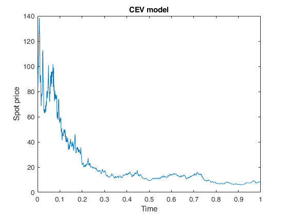
 Example of call of CEVmodel providing only price values.
Example of call of CEVmodel providing only price values.Generates spot prices for the CEV model at times t.
n=1000; dt=1/n;
t=0:dt:1; % discrete time grid
x=100; % initial price value
S=CEVmodel(t,x); % spot prices
plot(t,S)
xlabel('Time')
ylabel('Spot price')
title('CEV model')
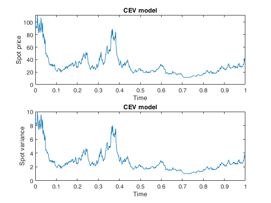
Example of call of CEVmodel providing both price and variance values.
Example of call of CEVmodel providing both price and variance values.Generates price and instantaneous variance values for the CEV model at times t.
n=1000; dt=1/n;
t=0:dt:1; % discrete time grid
x=100; % initial price value
[S,A]=CEVmodel(t,x); % spot prices and variance
subplot(2,1,1)
plot(t,S)
xlabel('Time')
ylabel('Spot price')
title('CEV model')
subplot(2,1,2)
plot(t,A)
xlabel('Time')
ylabel('Spot variance')
title('CEV model')