We assume our timeseries data are discrete observations from a diffusion
process following the It\^o stochastic differential equation
dx(t)= \sigma(t) \ dW(t) + b(t) \ dt,
where W is a Brownian motion on a filtered probability space. Let
\sigma and b be random processes, adapted to the Brownian filtration.
See the Reference for further mathematical details.
The squared diffusion coefficient \sigma^2(t) is called
instantaneous variance of the process x.
For any positive integer n, let {\cal S}_{n}:=\{ 0=t_{0}\leq \cdots
\leq t_{n}=T \} be the observation times. Moreover, let \delta_i(x):=
x(t_{i+1})-x(t_i) be the increments of x.
The Fourier estimator of the instantaneous variance for t \in (0,T),
is defined as
\widehat \sigma^2_{n,N,M}(t):= \sum_{|k|\leq M} \left(1- {|k|\over
M}\right) e^{{\rm i} {{2\pi}\over {T}} tk} c_k(\sigma^2_{n,N}),
where
c_k(\sigma^2_{n,N}):= {T \over {2N+1}}\sum_{|s|\leq N} c_s(dx_n)
c_{k-s}(dx_n),
where for any integer s, |s|\leq 2N, the discretized Fourier
coefficients of the increments are
c_s(dx_{n}):= {1\over {T}} \sum_{i=0}^{n-1} e^{-{\rm i} {{2\pi}\over {T}}
st_i}\delta_i(x).
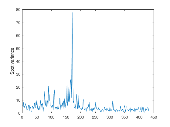
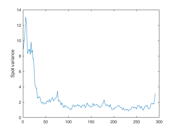
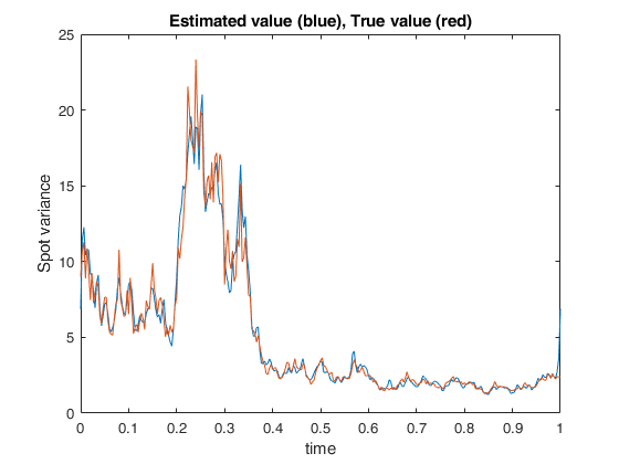
 Example of call of FE_spot_vol with just two input arguments.

