FE_int_vol_Fejer
FE_int_vol_Fejer computes the integrated variance from a diffusion process via the Fourier estimator using Fejer kernel
Description
FE_int_vol_Fejer computes the integrated variance of univariate timeseries data from a diffusion process by the Fourier estimator with Fejer kernel
FE_int_vol_Fejer called with optional input argument N.ivar
=FE_int_vol_Fejer(x,
t,
Name, Value)
Examples
 Example of call of FE_int_vol_Fejer with just two input arguments.
Example of call of FE_int_vol_Fejer with just two input arguments.The following example calculates the integrated variance from a vector x of discrete observations of a univariate diffusion process
n=1000;
dt=1/n; t=0:dt:1;
x=randn(n,1)*sqrt(dt); x=[0;cumsum(x)];
ivar=FE_int_vol_Fejer(x,t);
disp(['The value of the integrated variance is: ' num2str(ivar)])
The value of the integrated variance is: 0.97166
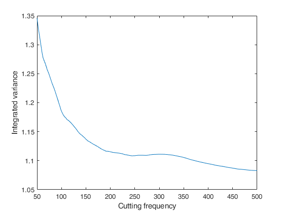
FE_int_vol_Fejer called with optional input argument N.
FE_int_vol_Fejer called with optional input argument N.Analysis of the change of the integrated variance estimates of a univariate diffusion process as a function of the different values of the cutting frequency.
n=1000;
dt=1/n; t=0:dt:1;
x=randn(n,1)*sqrt(dt); x=[0;cumsum(x)];
cuttingfreq=(50:500)';
l=length(cuttingfreq);
Ivar=zeros(l,1);
for i=1:l
ivar=FE_int_vol_Fejer(x,t,'N',cuttingfreq(i));
Ivar(i)=ivar;
end
plot(cuttingfreq,Ivar)
xlabel('Cutting frequency')
ylabel('Integrated variance')
Input Arguments
Output Arguments
More About
References
Mancino, M.E., Recchioni, M.C., Sanfelici, S. (2017), Fourier-Malliavin Volatility Estimation. Theory and Practice, "Springer Briefs in Quantitative Finance", Springer.