FSRaddt

FSRBbsb

FSRB

FSRB gives an automatic outlier detection procedure in Bayesian linear regression

expand all in page

Syntax

out=FSRB(y,X)example
out=FSRB(y,X,Name,Value)example

Description

example

out =FSRB(y, X) FSRB with all default options.

example

out =FSRB(y, X, Name, Value) FSRB with optional arguments.

Examples

expand all

FSRB with all default options.

Common part to the first examples: load Houses Price Dataset.

load hprice.txt;
n=size(hprice,1);
y=hprice(:,1);
X=hprice(:,2:5);
out=FSRB(y,X);

FSRB with optional arguments.

load hprice.txt;
n=size(hprice,1);
y=hprice(:,1);
X=hprice(:,2:5);
% set \beta components
beta0=0*ones(5,1);
beta0(2,1)=10;
beta0(3,1)=5000;
beta0(4,1)=10000;
beta0(5,1)=10000;
% \tau
s02=1/4.0e-8;
tau0=1/s02;
% R prior settings
R=2.4*eye(5);
R(2,2)=6e-7;
R(3,3)=.15;
R(4,4)=.6;
R(5,5)=.6;
R=inv(R);
% define a Bayes structure with previous data
n0=5;
bayes=struct;
bayes.R=R;
bayes.n0=n0;
bayes.beta0=beta0;
bayes.tau0=tau0;
intercept=true;
% function call
out=FSRB(y,X,'bayes',bayes,'msg',0,'plots',1,'init',round(n/2),'intercept', intercept)

out = 

  struct with fields:

     ListOut: [55 93 95 103 104 129 130 162 210 330 331 338 … ] (1×18 double)
    outliers: [55 93 95 103 104 129 130 162 210 330 331 338 … ] (1×18 double)
         mdr: [273×2 double]
          Un: [273×11 double]
        nout: [2×5 double]
        beta: [5×1 double]
       scale: 1.4951e+04
       class: 'FSRB'

Click here for the graphical output of this example (link to Ro.S.A. website).

Related Examples

expand all

Example on Fishery dataset (analysis with intercept).

nsamp is the number of subsamples to use in the frequentist analysis of first year, in order to find initial subset using LMS.

close all
nsamp=3000;
% threshold to be used to increase subset of good units
threshold=300;
bonflev=0.99; % Bonferroni confidence level to be used for first year
bonflevB=0.99; % Bonferroni confidence level to be used for subsequent years
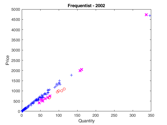
% Load 2002 Fishery dataset
Fishery2002=load('Fishery2002.txt');
y02=Fishery2002(:,3);
X02=Fishery2002(:,2);
n02=length(y02);
seq02=1:n02;
% frequentist Forward Search, 1st year
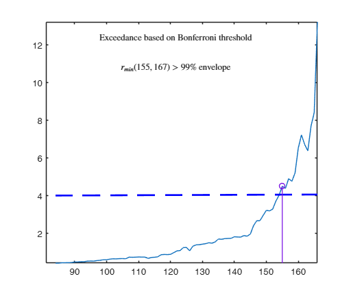
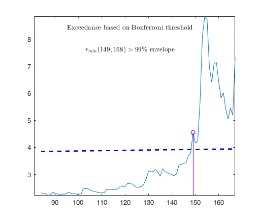
[out02]=FSR(y02,X02,'nsamp',nsamp,'plots',1,'msg',0,'init',round(n02*3/4),'bonflev',bonflev);
% In what follows
% g stands for good units
% i stand for intermediate units (i.e. units whose raw residual is smaller
% than threshold)
% o stands for outliers
% gi stands for good +intermediate units
% u02g = good units
% n02g = number of good units
u02g=setdiff(seq02,out02.ListOut);
n02g=length(u02g);
X02g=[ones(length(u02g),1) X02(u02g,:)];
y02g=y02(u02g);
% b02g = regression coefficients just using g units
b02g=X02g\y02g;
% res02 = squared raw residuals for all units using b02g
res02=(y02-[ones(length(X02),1) X02]*b02g).^2;
res02o=res02(out02.ListOut);
% sel= boolean vector which is true for the intermediate units
% (units whose squared residual is below the threshold)
sel=res02o<threshold^2;
% u02i = vector containing intermediate units (that is outliers whose
% residual is smaller than threshold)
u02i=out02.ListOut(sel);
% u02o = vector containing outliers whose residual is out of the threshold
u02o=out02.ListOut(~sel);
% u02gi = g + i units
if ~isempty(u02i)
u02gi=[u02g u02i];
else
u02gi=u02g;
end
% n02gi = number of good + intermediate units
n02gi=length(u02gi);
% plotting section
hold('off')
% good units, plotted as (+)
plot(X02(u02g)',y02(u02g)','Marker','+','LineStyle','none','Color','b')
hold('on')
% intermediate units plotted as (X)
plot(X02(u02i)',y02(u02i)','Marker','X','MarkerSize',9,'LineWidth',2,'LineStyle','none','Color','m')
% outliers, plotted as (O)
plot(X02(u02o)',y02(u02o)','Marker','o','LineStyle','none','Color','r')
xlabel('Quantity');
ylabel('Price');
title('Frequentist - 2002');
% S202gi = estimated of sigma^2 using g+i units
S202gi=sum(res02(u02gi))/(n02gi-2);
% X02gi = X matrix referred to good + intermediate units
X02gi=[ones(n02gi,1) X02(u02gi,:)];
% y02gi = y vector referred to good + intermediate units
y02gi=y02(u02gi);
% bayes = structure which contains prior information to be used in year
% 2003
bayes=struct;
bayes.beta0=b02g; % beta prior is beta based on g units
tau0=1/S202gi; % tau0 is based on g + i units
bayes.tau0=tau0;
R=X02g'*X02g; % R is based on g units
bayes.n0=n02gi; % n0 is based on g + i units
bayes.R=R;
% 2003
% Load 2003 Fishery dataset
Fishery2003=load('Fishery2003.txt');
y03=Fishery2003(:,3);
X03=Fishery2003(:,2);
n03=length(y03);
seq03=1:n03;
% Bayesian Forward Search, 2nd year
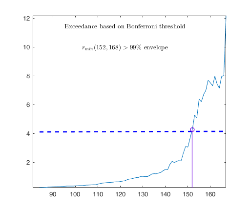
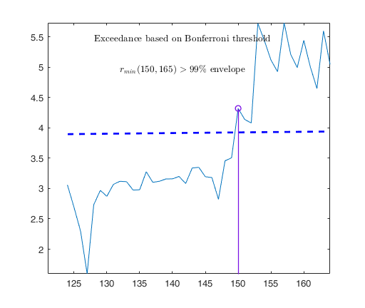
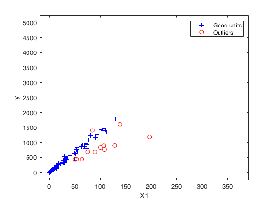
out03=FSRB(y03,X03,'bayes',bayes,'msg',0,'plots',1,'init',round(n03/2),'bonflev',bonflevB);
u03g=setdiff(seq03,out03.ListOut);
n03g=length(u03g);
% compute beta coefficient for year 2003 just using good units
X03g=[ones(n03g,1) X03(u03g,:)];
y03g=y03(u03g);
b03g=X03g\y03g;
res03=(y03-[ones(length(X03),1) X03]*b03g).^2;
res03o=res03(out03.ListOut);
sel=res03o<threshold^2;
% u03i = units to add to the good units subset (intermediate units)
u03i=out03.ListOut(sel);
% u03o =  outliers out of the threshold
u03o=out03.ListOut(~sel);
if ~isempty(u03i)
u03gi=[u03g u03i];
else
u03gi=u03g;
end
n03gi=length(u03gi);
X03gi=[ones(n03gi,1) X03(u03gi,:)];
y03gi=y03(u03gi,:);
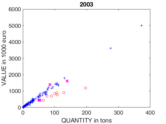
% plotting section
hold('off')
% good units, plotted as (+)
plot(X03(u03g)',y03(u03g)','Marker','+','LineStyle','none','Color','b')
hold('on')
% units below the threshold, plotted as (X)
plot(X03(u03i)',y03(u03i)','Marker','X','MarkerSize',9,'LineWidth',2,'LineStyle','none','Color','m')
% outliers, plotted as (O)
plot(X03(u03o)',y03(u03o)','Marker','o','LineStyle','none','Color','r')
set(gca,'FontSize',14)
xlabel('QUANTITY in tons')
ylabel('VALUE in 1000 euro')
title('2003');
% Definition of bayes structure (based on 2002 and 2003)
bayes=struct;
X02gX03g=[X02g; X03g];
y02gy03g=[y02g; y03g];
n02gn03g=n02g+n03g;
% b0203g prior estimate of beta for year 2004 is computed using good units
% for years 2002 and 2003
b0203g=X02gX03g\y02gy03g;
bayes.beta0=b0203g;
% R is just referred to good units for years 2002 and 2003
R=X02gX03g'*X02gX03g;
bayes.R=R;
% n0 is referred to g + i units in 2002 and 2003
bayes.n0=n02gi+n03gi;
X02giX03gi=[X02gi; X03gi];
y02giy03gi=[y02gi; y03gi];
% n02gin03gi = number of g+i units in 2002 and 2003
n02gin03gi=n02gi+n03gi;
% res = residuals for g+i units using b0203g
res=y02giy03gi-X02giX03gi*b0203g;
S203gi=sum(res.^2)/(n02gin03gi-2);
% estimate of tau is based on g + i units
tau0=1/S203gi;
bayes.tau0=tau0;
% Load 2004 Fishery dataset
Fishery2004=load('Fishery2004.txt');
y04=Fishery2004(:,3);
X04=Fishery2004(:,2);
n04=length(y04);
seq04=1:n04;
% Bayesian Forward Search, 3rd year
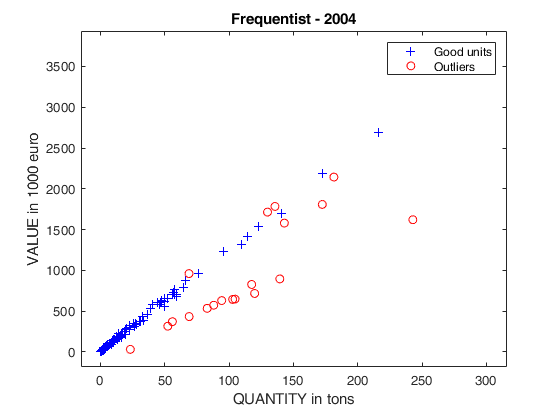
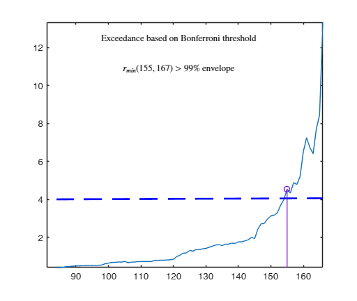
out04=FSRB(y04,X04,'bayes',bayes,'msg',0,'plots',1,'init',round(n04/2),'bonflev',bonflevB);
u04g=setdiff(seq04,out04.ListOut);
n04g=length(u04g);
X04g=[ones(n04g,1) X04(u04g,:)];
y04g=y04(u04g);
% b04g = beta based on good units for year 2004
b04g=X04g\y04g;
res04=(y04-[ones(length(X04),1) X04]*b04g).^2;
% res04o squared residuals for the tentative outliers
res04o=res04(out04.ListOut);
% we keep statistical units below the threshold
sel=res04o<threshold^2;
% u04i = units to add to the good units subset (intermediate units)
u04i=out04.ListOut(sel);
% u04o = units outliers out of the threshold
u04o=out04.ListOut(~sel);
if ~isempty(u04i)
u04gi=[u04g u04i];
else
u04gi=u04g;
end
n04gi=length(u04gi);
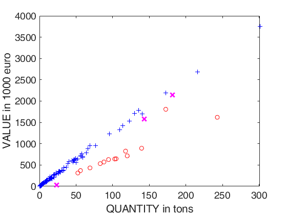
% plotting section
hold('off')
% good units, plotted as (+)
plot(X04(u04g)',y04(u04g)','Marker','+','LineStyle','none','Color','b')
hold('on')
% units below the threshold, plotted as (X)
plot(X04(u04i)',y04(u04i)','Marker','X','MarkerSize',9,'LineWidth',2,'LineStyle','none','Color','m')
% outliers, plotted as (O)
plot(X04(u04o)',y04(u04o)','Marker','o','LineStyle','none','Color','r')
set(gca,'FontSize',14)
xlabel('QUANTITY in tons')
ylabel('VALUE in 1000 euro')
% frequentist Forward Search, 3rd year
out04=FSR(y04,X04,'nsamp',nsamp,'plots',1,'msg',0,'init',round(n04/2),'bonflev',bonflev);
xlabel('QUANTITY in tons')
ylabel('VALUE in 1000 euro')
title('Frequentist - 2004');

Example on Fishery dataset (analysis without the intercept).

close all
% nsamp is the number of subsamples to use in the frequentist analysis of first
% year, in order to find initial subset using LMS.
nsamp=3000;
% threshold to be used to increase subset of good units
threshold=300;
bonflev=0.99; % Bonferroni confidence level
% Load 2002 Fishery dataset
Fishery2002=load('Fishery2002.txt');
y02=Fishery2002(:,3);
X02=Fishery2002(:,2);
n02=length(y02);
seq02=1:n02;
% frequentist Forward Search, 1st year (regression without intercept)
[out02]=FSR(y02,X02,'intercept',false,'nsamp',nsamp,'plots',1,'msg',0,'init',round(n02*3/4),'bonflev',bonflev);
% In what follows
% g stands for good units
% i stand for intermediate units (i.e. units whose raw residual is smaller
% than threshold)
% o stands for outliers
% gi stands for good +intermediate units
% u02g = good units
% n02g = number of good units
u02g=setdiff(seq02,out02.ListOut);
X02g=X02(u02g,:);
y02g=y02(u02g);
% b02g = regression coefficients just using g units
% Note that b02g is a scalar because the intercept has not been added
b02g=X02g\y02g;
% res02 = squared raw residuals for all units using b02g
res02=(y02-X02*b02g).^2;
res02o=res02(out02.ListOut);
% sel= boolean vector which is true for the intermediate units
% (units whose squared residual is below the threshold)
sel=res02o<threshold^2;
% u02i = vector containing intermediate units (that is outliers whose
% residual is smaller than threshold)
u02i=out02.ListOut(sel);
% u02gi = g + i units
if ~isempty(u02i)
u02gi=[u02g u02i];
else
u02gi=u02g;
end
% n02gi = number of good + intermediate units
n02gi=length(u02gi);
% S202gi = estimated of sigma^2 using g+i units
S202gi=sum(res02(u02gi))/(n02gi-1);
% bayes = structure which contains prior information to be used in year
% 2003
bayes=struct;
bayes.beta0=b02g; % beta prior is beta based on g units
tau0=1/S202gi; % tau0 is based on g + i units
bayes.tau0=tau0;
R=X02g'*X02g; % R is based on g units
bayes.n0=n02gi; % n0 is based on g + i units
bayes.R=R;
% 2003
% Load 2003 Fishery dataset
Fishery2003=load('Fishery2003.txt');
y03=Fishery2003(:,3);
X03=Fishery2003(:,2);
n03=length(y03);
% Run Bayesian Forward Search for the 2nd year using the prior based on
% the first year.
out03=FSRB(y03,X03,'bayes',bayes,'msg',0,'plots',1,'init',round(n03/2),'bonflev',bonflev,'intercept',false);

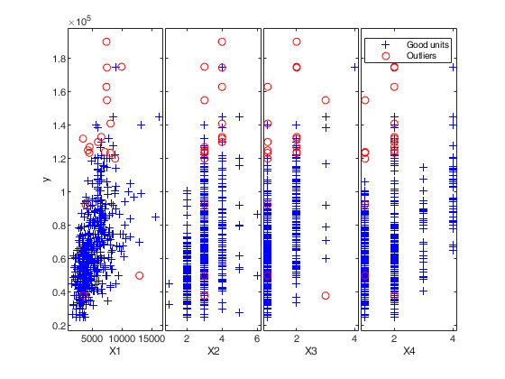
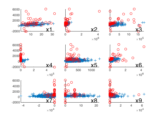
Outlier detection for Bank-Profit data.

XX=load('BankProfit.txt');
R=load('BankProfitR.txt');
X=XX(:,1:end-1);
y=XX(:,end);
% Load prior information
beta0=zeros(10,1);
beta0(1,1)=-0.5;
beta0(2,1)=9.1;         % Number of products (NUMPRO)
beta0(3,1)=0.001;       % direct revenues  (DIRREV)
beta0(4,1)=0.0002;      % indirect revenues   (INDREV)
beta0(5,1)=0.002;       %  savings accounts   SAVACC
beta0(6,1)=0.12;        %  number of operations   NUMOPE
beta0(7,1)=0.0004;      %  total amount of operations  TOTOPE
beta0(8,1)=-0.0004;     %  Bancomat POS
beta0(9,1)=1.3;         %  Number of cards   NUMCAR
beta0(10,1)=0.00004;    %  Amount in cards   TOTCAR
% \tau
s02=10000;
tau0=1/s02;
% number of obs in which prior was based
n0=1500;
bayes=struct;
bayes.R=R;
bayes.n0=n0;
bayes.beta0=beta0;
bayes.tau0=tau0;
intercept=true;
n=length(y);
out=FSRB(y,X,'bayes',bayes,'msg',1,'plots',1,...
'init',round(n/2),'xlim',[1700 1905],'ylim',[2 4]);
% Plot the outliers with a different symbol using a 3x3 layout.
selout=out.ListOut;
selin=setdiff(1:n,selout);
close all
% just in case user has additional function subtightplot
% http://www.mathworks.com/matlabcentral/fileexchange/39664-subtightplot
make_it_tight = false;
if make_it_tight == true && exist('subtightplot','file') ==2
subplot = @(m,n,p) subtightplot (m, n, p, [0.05 0.025], [0.1 0.01], [0.1 0.01]);
else
clear subplot;
end
% sel = panels in which yticks do not have to be removed
sel=[1 4 7];
miny=min(y);
maxy=max(y);
for j=1:9
subplot(3,3,j)
hold('on')
plot(X(selin,j),y(selin),'+')
plot(X(selout,j),y(selout),'ro')
ylim([miny maxy])
xlim([min(X(:,j)) max(X(:,j))])
if isempty(intersect(j,sel))
set(gca,'YTickLabel','')
end
% Add on the plot the variable name
text(0.75,0.1,['x' num2str(j)],'Units','normalized','FontSize',16)
end

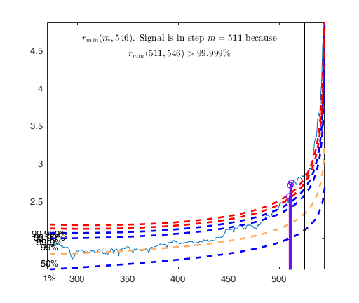
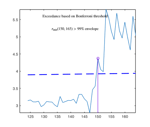
Observed curve of r_min is at least 10 times greater than 99.99% envelope
--------------------------------------------------
-------------------------
Signal detection loop
Tentative signal in central part of the search: step m=1830 because
rmin(1830,1903)>99.999%

-------------------
Signal validation exceedance of upper envelopes
Validated signal
-------------------------------
Start resuperimposing envelopes from step m=1829
Superimposition stopped because r_{min}(1851,1859)>99.9% envelope
Subsample of 1858 units is homogeneous
----------------------------
Final output
Number of units declared as outliers=45
Summary of the exceedances
           1          99         999        9999       99999
         838          77          76          73          73

Input Arguments

expand all

`y` — Response variable. Vector.

Response variable, specified as a vector of length n1, where n1 is the number of observations. Each entry in y is the response for the corresponding row of X.

Missing values (NaN's) and infinite values (Inf's) are allowed, since observations (rows) with missing or infinite values will automatically be excluded from the computations.

Data Types: single| double

`X` — Predictor variables. Matrix.

Matrix of explanatory variables (also called 'regressors') of dimension n1 x (p-1) where p denotes the number of explanatory variables including the intercept.

Rows of X represent observations, and columns represent variables. By default, there is a constant term in the model, unless you explicitly remove it using input option intercept, so do not include a column of 1s in X. Missing values (NaN's) and infinite values (Inf's) are allowed, since observations (rows) with missing or infinite values will automatically be excluded from the computations.

Remark: note that here we use symbol n1 instead of traditional symbol n because we want to better separate sample information coming from n1 values to prior information coming from n0 previous experiments.

Data Types: single| double

Name-Value Pair Arguments

Specify optional comma-separated pairs of Name,Value arguments. Name is the argument name and Value is the corresponding value. Name must appear inside single quotes (' '). You can specify several name and value pair arguments in any order as Name1,Value1,...,NameN,ValueN.

Example:

 'intercept',false
, bayes=struct;bayes.R=R;bayes.n0=n0;bayes.beta0=beta0;bayes.tau0=tau0;
, 'plots',1
, 'tag',{'plmdr' 'plyXplot'};
, 'init',100 starts monitoring from step m=100
, 'nocheck',true
, 'bivarfit',2
, 'multivarfit','1'
, 'labeladd','1'
, 'nameX',{'NameVar1','NameVar2'}
, 'namey','NameOfResponse'
, 'bonflev',0.99
, 'msg',1
, 'tag',{'plmdr' 'plyXplot'};

`intercept` —Indicator for constant term.true (default) | false.

Indicator for the constant term (intercept) in the fit, specified as the comma-separated pair consisting of 'Intercept' and either true to include or false to remove the constant term from the model.

Example: 'intercept',false

Data Types: boolean

`bayes` —Prior information.structure.

It contains the following fields

Value	Description
`beta0`	p-times-1 vector containing prior mean of \beta
`R`	p-times-p positive definite matrix which can be interpreted as X0'X0 where X0 is a n0 x p matrix coming from previous experiments (assuming that the intercept is included in the model). The prior distribution of $\tau_0$ is a gamma distribution with parameters $a_0$ and $b_0$ , that is $p(\tau_0) \propto \tau^{a_0-1} \exp (-b_0 \tau) \qquad E(\tau_0) = a_0/b_0$
`tau0`	scalar. Prior estimate of $\tau=1/ \sigma^2 =a_0/b_0$
`n0`	scalar. Sometimes it helps to think of the prior information as coming from n0 previous experiments. Therefore we assume that matrix X0 (which defines R), was made up of n0 observations. REMARK if structure bayes is not supplied the default values which are used are. beta0= zeros(p,1): Vector of zeros. R=eye(p): Identity matrix. tau0=1/1e+6: Very large value for the prior variance, that is a very small value for tau0. n0=1: just one prior observation. $\beta$ is assumed to have a normal distribution with mean $\beta_0$ and (conditional on $\tau_0$ ) covariance $(1/\tau_0) (X_0'X_0)^{-1}$ . $\beta \sim N( \beta_0, (1/\tau_0) (X_0'X_0)^{-1} )$

Example: bayes=struct;bayes.R=R;bayes.n0=n0;bayes.beta0=beta0;bayes.tau0=tau0;

Data Types: double

`plots` —Plot on the screen.scalar.

If plots=1 (default) the plot of minimum deletion residual with envelopes based on n observations and the scatterplot matrix with the outliers highlighted is produced.

If plots=2 the user can also monitor the intermediate plots based on envelope superimposition.

Else no plot is produced.

Example: 'plots',1

Data Types: double

`tag` —tags to the plots which are created.character | cell array of characters.

This option enables to add a tag to the plots which are created. The default tag names are: fsr_mdrplot for the plot of mdr based on all the observations;

fsr_yXplot for the plot of y against each column of X with the outliers highlighted;

fsr_resuperplot for the plot of resuperimposed envelopes. The first plot with 4 panel of resuperimposed envelopes has tag fsr_resuperplot1, the second fsr_resuperplot2 ...

If tag is character or a cell of characters of length 1, it is possible to specify the tag for the plot of mdr based on all the observations;

If tag is a cell of length 2 it is possible to control both the tag for the plot of mdr based on all the observations and the tag for the yXplot with outliers highlighted.

If tag is a cell of length 3 the third element specifies the names of the plots of resuperimposed envelopes.

Example: 'tag',{'plmdr' 'plyXplot'};

Data Types: char or cell

`init` —Search initialization.scalar.

scalar which specifies the initial subset size to start monitoring exceedances of minimum deletion residual, if init is not specified it set equal to: p+1, if the sample size is smaller than 40;

min(3*p+1,floor(0.5*(n+p+1))), otherwise.

Example: 'init',100 starts monitoring from step m=100

Data Types: double

`nocheck` —Check input arguments.boolean.

If nocheck is equal to true no check is performed on matrix y and matrix X. Notice that y and X are left unchanged. In other words the additional column of ones for the intercept is not added. As default nocheck=false.

Example: 'nocheck',true

Data Types: boolean

`bivarfit` —Superimpose bivariate least square lines.character.

This option adds one or more least square lines, based on SIMPLE REGRESSION of y on Xi, to the plots of y|Xi.

bivarfit = '' is the default: no line is fitted.

bivarfit = '1' fits a single ols line to all points of each bivariate plot in the scatter matrix y|X.

bivarfit = '2' fits two ols lines: one to all points and another to the group of the genuine observations. The group of the potential outliers is not fitted.

bivarfit = '0' fits one ols line to each group. This is useful for the purpose of fitting mixtures of regression lines.

bivarfit = 'i1' or 'i2' or 'i3' etc.

fits an ols line to a specific group, the one with index 'i' equal to 1, 2, 3 etc. Again, useful in case of mixtures.

Example: 'bivarfit',2

Data Types: char

`multivarfit` —Superimpose multivariate least square lines.character.

This option adds one or more least square lines, based on MULTIVARIATE REGRESSION of y on X, to the plots of y|Xi.

multivarfit = '' is the default: no line is fitted.

multivarfit = '1' fits a single ols line to all points of each bivariate plot in the scatter matrix y|X. The line added to the scatter plot y|Xi is avconst + Ci*Xi, where Ci is the coefficient of Xi in the multivariate regression and avconst is the effect of all the other explanatory variables different from Xi evaluated at their centroid (that is overline{y}'C)) multivarfit = '2' equal to multivarfit ='1' but this time we also add the line based on the group of unselected observations (i.e. the normal units).

Example: 'multivarfit','1'

Data Types: char

`labeladd` —Add outlier labels in plot.character.

If this option is '1', we label the outliers with the unit row index in matrices X and y. The default value is labeladd='', i.e. no label is added.

Example: 'labeladd','1'

Data Types: char

`nameX` —Add variable labels in plot.cell array of strings.

Cell array of strings of length p containing the labels of the variables of the regression dataset. If it is empty (default) the sequence X1, ..., Xp will be created automatically

Example: 'nameX',{'NameVar1','NameVar2'}

Data Types: cell

`namey` —Add response label.character.

Character containing the label of the response

Example: 'namey','NameOfResponse'

Data Types: char

`ylim` —Control y scale in plot.vector.

Vector with two elements controlling minimum and maximum on the y axis. Default value is '' (automatic scale)

Example: 'ylim','[0,10]' sets the minimum value to 0 and the max to 10 on the y axis

Data Types: double

`xlim` —Control x scale in plot.vector.

Vector with two elements controlling minimum and maximum on the x axis. Default value is '' (automatic scale)

Example: 'xlim','[0,10]' sets the minimum value to 0 and the max to 10 on the x axis

Data Types: double

`bonflev` —Signal to use to identify outliers.scalar.

Option to be used if the distribution of the data is strongly non normal and, thus, the general signal detection rule based on consecutive exceedances cannot be used. In this case bonflev can be: - a scalar smaller than 1 which specifies the confidence level for a signal and a stopping rule based on the comparison of the minimum MD with a Bonferroni bound. For example, if bonflev=0.99, the procedure stops when the trajectory exceeds for the first time the 99% bonferroni bound.

- A scalar value greater than 1. In this case the procedure stops when the residual trajectory exceeds for the first time this value.

Default value is '', which means to rely on general rules based on consecutive exceedances.

Example: 'bonflev',0.99

Data Types: double

`msg` —Level of output to display.scalar.

Scalar which controls whether to display or not messages on the screen If msg==1 (default) messages are displayed on the screen about step in which signal took place and ....

else no message is displayed on the screen

Example: 'msg',1

Data Types: double

`tag` —tags to the plots which are created.character | cell array of characters.

This option enables to add a tag to the plots which are created. The default tag names are: fsrb_mdrplot for the plot of mdr based on all the observations;

fsrb_yXplot for the plot of y against each column of X with the outliers highlighted;

fsrb_resuperplot for the plot of resuperimposed envelopes. The first plot with 4 panel of resuperimposed envelopes has tag fsrb_resuperplot1, the second fsrb_resuperplot2 ...

If tag is character or a cell of characters of length 1, it is possible to specify the tag for the plot of mdr based on all the observations;

If tag is a cell of length 2 it is possible to control both the tag for the plot of mdr based on all the observations and the tag for the yXplot with outliers highlighted.

If tag is a cell of length 3 the third element specifies the names of the plots of resuperimposed envelopes.

Example: 'tag',{'plmdr' 'plyXplot'};

Data Types: char or cell array of characters

Output Arguments

expand all

`out` — description Structure

Structure which contains the following fields

Value	Description
`ListOut`	k x 1 vector containing the list of the units declared as outliers or empty if the sample is homogeneous. This field in future releases will be deleted because it will be replaced by out.outliers.
`outliers`	k x 1 vector containing the list of the units declared as outliers or empty if the sample is homogeneous.
`beta`	p-by-1 vector containing the posterior mean of $\beta$ (regression coefficients), $\beta = (cR + X'X)^{-1} (cR*\beta_0 + X'y)$ in step $n-k$
`scale`	scalar. This is the reciprocal of the square root of the posterior estimate of $\tau$ in step $n-k$
`mdr`	(n-init) x 2 matrix: 1st col = fwd search index; 2nd col = value of Bayesian minimum deletion residual in each step of the fwd search.
`Un`	(n-init) x 11 Matrix which contains the unit(s) included in the subset at each step of the fwd search. REMARK: in every step the new subset is compared with the old subset. Un contains the unit(s) present in the new subset but not in the old one. Un(1,2), for example, contains the unit included in step init+1. Un(end,2) contains the units included in the final step of the search.
`nout`	2 x 5 matrix containing the number of times mdr went out of particular quantiles. First row contains quantiles 1 99 99.9 99.99 99.999. Second row contains the frequency distribution.
`constr`	This output is produced only if the search found at a certain step a non singular matrix X. In this case the search runs in a constrained mode, that is including the units which produced a singular matrix in the last n-constr steps. out.constr is a vector which contains the list of units which produced a singular X matrix
`class`	'FSRB'.

References

Chaloner, K. and Brant, R. (1988), A Bayesian Approach to Outlier Detection and Residual Analysis, "Biometrika", Vol. 75, pp. 651-659.

Riani, M., Corbellini, A. and Atkinson, A.C. (2018), Very Robust Bayesian Regression for Fraud Detection, "International Statistical Review", http://dx.doi.org/10.1111/insr.12247

Atkinson, A.C., Corbellini, A. and Riani, M., (2017), Robust Bayesian Regression with the Forward Search: Theory and Data Analysis, "Test", Vol. 26, pp. 869-886, https://doi.org/10.1007/s11749-017-0542-6

Documentation

FSRB

Syntax

Description

Examples

FSRB with all default options.

FSRB with optional arguments.

Related Examples

Example on Fishery dataset (analysis with intercept).

Example on Fishery dataset (analysis without the intercept).

Outlier detection for Bank-Profit data.

Input Arguments

`y` — Response variable. Vector.

`X` — Predictor variables. Matrix.

Name-Value Pair Arguments

`intercept` —Indicator for constant term.true (default) | false.

`bayes` —Prior information.structure.

`plots` —Plot on the screen.scalar.

`tag` —tags to the plots which are created.character | cell array of characters.

`init` —Search initialization.scalar.

`nocheck` —Check input arguments.boolean.

`bivarfit` —Superimpose bivariate least square lines.character.

`multivarfit` —Superimpose multivariate least square lines.character.

`labeladd` —Add outlier labels in plot.character.

`nameX` —Add variable labels in plot.cell array of strings.

`namey` —Add response label.character.

`ylim` —Control y scale in plot.vector.

`xlim` —Control x scale in plot.vector.

`bonflev` —Signal to use to identify outliers.scalar.

`msg` —Level of output to display.scalar.

`tag` —tags to the plots which are created.character | cell array of characters.

Output Arguments

`out` — description Structure

References

See Also

Documentation

FSRB

Syntax

Description

Examples

FSRB with all default options.

FSRB with optional arguments.

Related Examples

Example on Fishery dataset (analysis with intercept).

Example on Fishery dataset (analysis without the intercept).

Outlier detection for Bank-Profit data.

Input Arguments

y — Response variable. Vector.

X — Predictor variables. Matrix.

Name-Value Pair Arguments

intercept —Indicator for constant term.true (default) | false.

bayes —Prior information.structure.

plots —Plot on the screen.scalar.

tag —tags to the plots which are created.character | cell array of characters.

init —Search initialization.scalar.

nocheck —Check input arguments.boolean.

bivarfit —Superimpose bivariate least square lines.character.

multivarfit —Superimpose multivariate least square lines.character.

labeladd —Add outlier labels in plot.character.

nameX —Add variable labels in plot.cell array of strings.

namey —Add response label.character.

ylim —Control y scale in plot.vector.

xlim —Control x scale in plot.vector.

bonflev —Signal to use to identify outliers.scalar.

msg —Level of output to display.scalar.

tag —tags to the plots which are created.character | cell array of characters.

Output Arguments

out — description Structure

References

See Also

`y` — Response variable. Vector.

`X` — Predictor variables. Matrix.

`intercept` —Indicator for constant term.true (default) | false.

`bayes` —Prior information.structure.

`plots` —Plot on the screen.scalar.

`tag` —tags to the plots which are created.character | cell array of characters.

`init` —Search initialization.scalar.

`nocheck` —Check input arguments.boolean.

`bivarfit` —Superimpose bivariate least square lines.character.

`multivarfit` —Superimpose multivariate least square lines.character.

`labeladd` —Add outlier labels in plot.character.

`nameX` —Add variable labels in plot.cell array of strings.

`namey` —Add response label.character.

`ylim` —Control y scale in plot.vector.

`xlim` —Control x scale in plot.vector.

`bonflev` —Signal to use to identify outliers.scalar.

`msg` —Level of output to display.scalar.

`tag` —tags to the plots which are created.character | cell array of characters.

`out` — description Structure