
|
FSRBbsb |
FSRBmdr |
 |
FSRBeda
FSRBeda enables to monitor several quantities in each step of the Bayesian search
Description
Examples
Related Examples
 Plot posterior estimates of beta and sigma2.
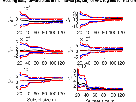
Plot posterior estimates of beta and sigma2.Plot posterior estimates of beta and sigma2 in the interval (subset size) [20 125].
% In this example, for the house price data, we monitor the forward plots
% of the parameters of the linear model, adding 95% and 99% HPD
% regions. The first 8 panels refer to the elements of $\beta_1$
% and the bottom right-hand panel refer to the estimate of sigma2.
% The horizontal lines correspond to prior values.
% The vertical lines refer to the step prior to the introduction of the first outlier
% init = point to start monitoring diagnostics along the FS
% run routine FSRB in order to find the outliers automatically.
load hprice.txt;
% setup parameters
n=size(hprice,1);
y=hprice(:,1);
X=hprice(:,2:5);
bayes=struct;
n0=5;
bayes.n0=n0;
% set \beta components
beta0=0*ones(5,1);
beta0(2,1)=10;
beta0(3,1)=5000;
beta0(4,1)=10000;
beta0(5,1)=10000;
bayes.beta0=beta0;
% \tau
s02=1/4.0e-8;
tau0=1/s02;
bayes.tau0=tau0;
% R prior settings
R=2.4*eye(5);
R(2,2)=6e-7;
R(3,3)=.15;
R(4,4)=.6;
R(5,5)=.6;
R=inv(R);
bayes.R=R;
outBA=FSRB(y,X,'bayes',bayes', 'plots',0);
dout=n-length(outBA.ListOut);
% init = initial point to start monitoring
init=20;
xlimL=init; % lower value of xlim
xlimU=125;  % upper value of xlim
outBAeda=FSRBeda(y,X,'bayes',bayes,'init',init, 'conflev', [0.95 0.99]);
% Set font size, line width and line style
figure;
lwd=2.5;
FontSize=14;
linst={'-','--',':','-.','--',':'};
for j=1:5
my_subplot=subplot(3,2,j);
hold('on')
% plot 95% and 99% HPD  trajectories
plot(outBAeda.beta1(:,1),outBAeda.beta1HPD(:,1:2,j),'LineStyle',linst{4},'LineWidth',lwd,'Color','b')
plot(outBAeda.beta1(:,1),outBAeda.beta1HPD(:,3:4,j),'LineStyle',linst{4},'LineWidth',lwd,'Color','r')
% plot posterior estimate of beta1_j
plot(outBAeda.beta1(:,1),outBAeda.beta1(:,j+1)','LineStyle',linst{1},'LineWidth',lwd,'Color','k')
% Add the horizontal line which corresponds to prior values
xL = get(my_subplot,'XLim');
line(xL,[beta0(j) beta0(j)],'Color','r','LineWidth',lwd);
% Set ylim
ylimU=max([outBAeda.beta1HPD(:,4,j); beta0(j)]);
ylimL=min([outBAeda.beta1HPD(:,3,j); beta0(j)]);
ylim([ylimL ylimU])
% Add vertical line in correspondence of the step prior to the
% entry of the first outlier
line([dout; dout],[ylimL; ylimU],'Color','r','LineWidth',lwd);
% Set xlim
xlim([xlimL xlimU]);
ylabel(['$\hat{\beta_' num2str(j-1) '}$'],'Interpreter','LaTeX','FontSize',20,'rot',-360);
set(gca,'FontSize',FontSize);
if j>4
xlabel('Subset size m','FontSize',FontSize);
end
end
% Subplot associated with the monitoring of sigma^2
subplot(3,2,6);
%figure()
hold('on')
% 99%
plot(outBAeda.sigma21HPD(:,1),outBAeda.sigma21HPD(:,4:5),'LineStyle',linst{4},'LineWidth',lwd,'Color','r')
% 95%
plot(outBAeda.sigma21HPD(:,1),outBAeda.sigma21HPD(:,2:3),'LineStyle',linst{2},'LineWidth',lwd,'Color','b')
% Plot 1\/tau1
plot(outBAeda.S21(:,1),1./outBAeda.S21(:,3),'LineWidth',lwd,'Color','k')
ylabel('$\hat{\sigma}^2$','Interpreter','LaTeX','FontSize',20,'rot',-360);
set(gca,'FontSize',FontSize);
% Set ylim
ylimU=max([outBAeda.sigma21HPD(:,5); s02]);
ylimL=min([outBAeda.sigma21HPD(:,4); s02]);
ylim([ylimL ylimU])
% Set xlim
xlim([xlimL xlimU]);
xL = get(my_subplot,'XLim');
% Add the horizontal line which corresponds to prior value of $\sigma^2$
line(xL,[s02 s02],'Color','r','LineWidth',lwd);
% Add vertical line in correspondence of the step prior to the
% entry of the first outlier
line([dout; dout],[ylimL; ylimU],'Color','r','LineWidth',lwd);
xlabel('Subset size m','FontSize',FontSize);
% Add multiple title
suplabel(['Housing data; forward plots in the interval ['...
num2str(xlimL) ',' num2str(xlimU) ...
']  of HPD regions for \beta and \sigma^2'],'t');
Observed curve of r_min is at least 10 times greater than 99.99% envelope
--------------------------------------------------
-------------------------
Signal detection loop
Tentative signal in central part of the search: step m=511 because
rmin(511,546)>99.99% and rmin(510,546)>99.99% and rmin(512,546)>99.99%
rmin(511,546)>99.999%

-------------------
Signal validation exceedance of upper envelopes
Validated signal
-------------------------------
Start resuperimposing envelopes from step m=510
Superimposition stopped because r_{min}(512,529)>99.9% envelope
Subsample of 528 units is homogeneous
----------------------------
Final output
Number of units declared as outliers=18
Summary of the exceedances
           1          99         999        9999       99999
          10          64          48          38          29

m=100
m=200
m=300
m=400
m=500

Plot posterior estimates of beta and sigma2 in the last steps.
Plot posterior estimates of beta and sigma2 in the last steps.Plot posterior estimates of beta and sigma2 in the interval (subset size) [250 n+1].
% In this example for the house price data we monitor the forward plots
% of the parameters of the linear model adding 95% and 99% HPD
% regions. The first 8 panels refer to the elements of $\beta_1$
% and the bottom right-hand panel refer to the estimate of sigma2.
% The horizontal lines correspond to prior values.
% The vertical lines refer to the step prior to the introduction of the first outlier
% init = point to start monitoring diagnostics along the FS
% run routine FSRB in order to find the outliers automatically
load hprice.txt;
% setup parameters
n=size(hprice,1);
y=hprice(:,1);
X=hprice(:,2:5);
bayes=struct;
n0=5;
bayes.n0=n0;
% set \beta components
beta0=0*ones(5,1);
beta0(2,1)=10;
beta0(3,1)=5000;
beta0(4,1)=10000;
beta0(5,1)=10000;
bayes.beta0=beta0;
% \tau
s02=1/4.0e-8;
tau0=1/s02;
bayes.tau0=tau0;
% R prior settings
R=2.4*eye(5);
R(2,2)=6e-7;
R(3,3)=.15;
R(4,4)=.6;
R(5,5)=.6;
R=inv(R);
bayes.R=R;
% Automatic outlier detection procedure.
outBA=FSRB(y,X,'bayes',bayes', 'plots',0);
dout=n-length(outBA.ListOut);
% init = initial point to start monitoring
init=250;
xlimL=init; % lower value fo xlim
xlimU=n+1;  % upper value of xlim
out=FSRBeda(y,X,'bayes',bayes,'init',init, 'conflev', [0.95 0.99]);
% Set font size, line width and line style
figure;
lwd=2.5;
FontSize=14;
linst={'-','--',':','-.','--',':'};
for j=1:5
my_subplot=subplot(3,2,j);
hold('on')
% plot 95% and 99% HPD  trajectories
plot(out.beta1(:,1),out.beta1HPD(:,1:2,j),'LineStyle',linst{4},'LineWidth',lwd,'Color','b')
plot(out.beta1(:,1),out.beta1HPD(:,3:4,j),'LineStyle',linst{4},'LineWidth',lwd,'Color','r')
% plot posterior estimate of beta1_j
plot(out.beta1(:,1),out.beta1(:,j+1)','LineStyle',linst{1},'LineWidth',lwd,'Color','k')
% Add the horizontal line which corresponds to prior values
xL = get(my_subplot,'XLim');
line(xL,[beta0(j) beta0(j)],'Color','r','LineWidth',lwd);
% Set ylim
ylimU=max([out.beta1HPD(:,4,j); beta0(j)]);
ylimL=min([out.beta1HPD(:,3,j); beta0(j)]);
ylim([ylimL ylimU])
% Set xlim
xlim([xlimL xlimU]);
% Add vertical line in correspondence of the step prior to the
% entry of the first outlier
line([dout; dout],[ylimL; ylimU],'Color','r','LineWidth',lwd);
ylabel(['$\hat{\beta_' num2str(j-1) '}$'],'Interpreter','LaTeX','FontSize',20,'rot',-360);
set(gca,'FontSize',FontSize);
if j>4
xlabel('Subset size m','FontSize',FontSize);
end
end
% Subplot associated with the monitoring of sigma^2
subplot(3,2,6);
%figure()
hold('on')
% 99%
plot(out.sigma21HPD(:,1),out.sigma21HPD(:,4:5),'LineStyle',linst{4},'LineWidth',lwd,'Color','r')
% 95%
plot(out.sigma21HPD(:,1),out.sigma21HPD(:,2:3),'LineStyle',linst{2},'LineWidth',lwd,'Color','b')
% Plot 1/tau1
plot(out.S21(:,1),1./out.S21(:,3),'LineWidth',lwd,'Color','k')
ylabel('$\hat{\sigma}^2$','Interpreter','LaTeX','FontSize',20,'rot',-360);
set(gca,'FontSize',FontSize);
% Set ylim
ylimU=max([out.sigma21HPD(:,5); s02]);
ylimL=min([out.sigma21HPD(:,4); s02]);
ylim([ylimL ylimU])
% Set xlim
xlim([xlimL xlimU]);
xL = get(my_subplot,'XLim');
% Add the horizontal line which corresponds to prior value of $\sigma^2$
line(xL,[s02 s02],'Color','r','LineWidth',lwd);
% Add vertical line in correspondence of the step prior to the
% entry of the first outlier
line([dout; dout],[ylimL; ylimU],'Color','r','LineWidth',lwd);
xlabel('Subset size m','FontSize',FontSize);
% Add multiple title
suplabel(['Housing data; forward plots in the interval ['...
num2str(xlimL) ',' num2str(xlimU) ...
']  of HPD regions for \beta and \sigma^2'],'t');
Observed curve of r_min is at least 10 times greater than 99.99% envelope
--------------------------------------------------
-------------------------
Signal detection loop
Tentative signal in central part of the search: step m=511 because
rmin(511,546)>99.99% and rmin(510,546)>99.99% and rmin(512,546)>99.99%
rmin(511,546)>99.999%

-------------------
Signal validation exceedance of upper envelopes
Validated signal
-------------------------------
Start resuperimposing envelopes from step m=510
Superimposition stopped because r_{min}(512,529)>99.9% envelope
Subsample of 528 units is homogeneous
----------------------------
Final output
Number of units declared as outliers=18
Summary of the exceedances
           1          99         999        9999       99999
          10          64          48          38          29

m=100
m=200
m=300
m=400
m=500
Input Arguments
Output Arguments
References
Chaloner, K. and Brant, R. (1988), A Bayesian Approach to Outlier Detection and Residual Analysis, "Biometrika", Vol. 75, pp. 651-659.
Riani, M., Corbellini, A. and Atkinson, A.C. (2018), Very Robust Bayesian Regression for Fraud Detection, "International Statistical Review", http://dx.doi.org/10.1111/insr.12247
Atkinson, A.C., Corbellini, A. and Riani, M., (2017), Robust Bayesian Regression with the Forward Search: Theory and Data Analysis, "Test", Vol. 26, pp. 869-886, https://doi.org/10.1007/s11749-017-0542-6
|
|
FSRBbsb |
FSRBmdr |
|
|
|
Functions |
|
• The developers of the toolbox • The forward search group • Terms of Use • Acknowledgments