
|
FSRHeda |
FSRinvmdr |
 |
FSRHmdr
FSRHmdr computes minimum deletion residual and other basic linear regression quantities in each step of the heteroskedastic search
Syntax
mdr=FSRHmdr(y,X,Z,bsb)examplemdr=FSRHmdr(y,X,Z,bsb,Name,Value)example[mdr,Un]=FSRHmdr(___)example[mdr,Un,BB]=FSRHmdr(___)example[mdr,Un,BB,Bgls]=FSRHmdr(___)example[mdr,Un,BB,Bgls,S2]=FSRHmdr(___)example[mdr,Un,BB,Bgls,S2,Hetero]=FSRHmdr(___)example[mdr,Un,BB,Bgls,S2,Hetero,WEI]=FSRHmdr(___)example
Description
Examples
 FSRHmdr with all default options.
FSRHmdr with all default options.Common part to all examples: load tradeH dataset (used in the paper ART).
XX=load('tradeH.txt');
y=XX(:,2);
X=XX(:,1);
X=X./max(X);
Z=log(X);
mdr=FSRHmdr(y,X,Z,0);
Warning: interchange greater than 10 when m=22
Number of units which entered=21
Warning: interchange greater than 10 when m=24
Number of units which entered=14
Warning: Matrix is singular, close to singular or badly scaled. Results may be
inaccurate. RCOND = NaN.
Warning: interchange greater than 10 when m=25
Number of units which entered=24
Warning: interchange greater than 10 when m=26
Number of units which entered=27
Warning: interchange greater than 10 when m=165
Number of units which entered=11
Warning: interchange greater than 10 when m=166
Number of units which entered=39
Warning: interchange greater than 10 when m=167
Number of units which entered=11
Warning: interchange greater than 10 when m=168
Number of units which entered=15
Warning: interchange greater than 10 when m=169
Number of units which entered=16
Warning: interchange greater than 10 when m=170
Number of units which entered=13
Warning: interchange greater than 10 when m=171
Number of units which entered=11
Warning: interchange greater than 10 when m=172
Number of units which entered=11
Warning: interchange greater than 10 when m=180
Number of units which entered=12
Warning: interchange greater than 10 when m=181
Number of units which entered=25
Warning: interchange greater than 10 when m=182
Number of units which entered=15
Warning: interchange greater than 10 when m=183
Number of units which entered=18
Warning: interchange greater than 10 when m=225
Number of units which entered=15
Warning: interchange greater than 10 when m=482
Number of units which entered=26
Warning: interchange greater than 10 when m=483
Number of units which entered=11
Warning: interchange greater than 10 when m=484
Number of units which entered=12
Warning: interchange greater than 10 when m=485
Number of units which entered=12
Warning: interchange greater than 10 when m=486
Number of units which entered=11
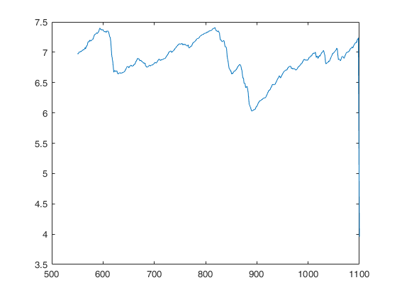
Monitoring the estimates of the scedastic equation.
Monitoring the estimates of the scedastic equation.With plot of the \alpha parameter.
XX=load('tradeH.txt');
y=XX(:,2);
X=XX(:,1);
X=X./max(X);
Z=log(X);
[mdr,Un,BB,Bols,S2,Hetero]=FSRHmdr(y,X,Z,0,'init',round(length(y)/2));
plot(Hetero(:,1),Hetero(:,2))
Warning: Maximum number of iterations has been reached without convergence
Input Arguments
Output Arguments
References
Atkinson, A.C., Riani, M. and Torti, F. (2016), Robust methods for heteroskedastic regression, "Computational Statistics and Data Analysis", Vol. 104, pp. 209-222, http://dx.doi.org/10.1016/j.csda.2016.07.002 [ART]