
|
FSRtsbsb |
funnelchart |
 |
FSRtsmdr
FSRtsmdr computes minimum deletion residual for time series models in each step of the search
Syntax
Examples
 Analyze units entering the search in the final steps.
Analyze units entering the search in the final steps.Common part to all examples: load airline dataset.
% 1949 1950 1951 1952 1953 1954 1955 1956 1957 1958 1959 1960
y = [112 115 145 171 196 204 242 284 315 340 360 417 % Jan
118 126 150 180 196 188 233 277 301 318 342 391 % Feb
132 141 178 193 236 235 267 317 356 362 406 419 % Mar
129 135 163 181 235 227 269 313 348 348 396 461 % Apr
121 125 172 183 229 234 270 318 355 363 420 472 % May
135 149 178 218 243 264 315 374 422 435 472 535 % Jun
148 170 199 230 264 302 364 413 465 491 548 622 % Jul
148 170 199 242 272 293 347 405 467 505 559 606 % Aug
136 158 184 209 237 259 312 355 404 404 463 508 % Sep
119 133 162 191 211 229 274 306 347 359 407 461 % Oct
104 114 146 172 180 203 237 271 305 310 362 390 % Nov
118 140 166 194 201 229 278 306 336 337 405 432 ]; % Dec
y=(y(:));
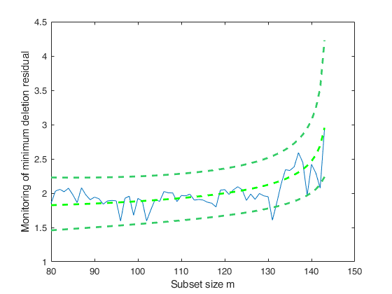
% Compute minimum deletion residual and analyze the units entering
% subset in each step of the fwd search (matrix Un). As is well known,
% the FS provides an ordering of the data from those most in agreement
% with a suggested model (which enter the first steps) to those least in
% agreement with it (which are included in the final steps).
% Set up a personalized model.
model=struct;
model.trend=1; % linear trend
model.s=12; % monthly time series
model.seasonal=104; % four harmonics with time varying seasonality
% Choose step to start monitoring.
init=80;
[mdr,Un,BB,Bols,S2,Exflag]=FSRtsmdr(y,0,'model',model,'init',80,'plots',1);
% Check if there was convergence in all step which were monitored.
if min(Exflag(:,2))<1
disp('Warning: in some steps there was not convergence')
else
disp('Convergence obtained in all steps')
end
% Check the last two units which are included in the last two steps.
disp(Un(end-1:end,:))
Convergence obtained in all steps
   143   139   NaN   NaN   NaN   NaN   NaN   NaN   NaN   NaN   NaN
   144   142   NaN   NaN   NaN   NaN   NaN   NaN   NaN   NaN   NaN
Store units forming subsets in selected steps.
Store units forming subsets in selected steps.In this example the units forming subset are stored just for selected steps.
%   1949 1950 1951 1952 1953 1954 1955 1956 1957 1958 1959 1960
y = [112  115  145  171  196  204  242  284  315  340  360  417    % Jan
118  126  150  180  196  188  233  277  301  318  342  391    % Feb
132  141  178  193  236  235  267  317  356  362  406  419    % Mar
129  135  163  181  235  227  269  313  348  348  396  461    % Apr
121  125  172  183  229  234  270  318  355  363  420  472    % May
135  149  178  218  243  264  315  374  422  435  472  535    % Jun
148  170  199  230  264  302  364  413  465  491  548  622    % Jul
148  170  199  242  272  293  347  405  467  505  559  606    % Aug
136  158  184  209  237  259  312  355  404  404  463  508    % Sep
119  133  162  191  211  229  274  306  347  359  407  461    % Oct
104  114  146  172  180  203  237  271  305  310  362  390    % Nov
118  140  166  194  201  229  278  306  336  337  405  432 ]; % Dec
y=(y(:));
model=struct;
model.trend=1;              % linear trend
model.s=12;                 % monthly time series
model.seasonal=104;         % four harmonics with time varying seasonality
init=80;
[mdr,Un,BB,Bols,S2] =FSRtsmdr(y,0,'model',model,'init',80,'bsbsteps',[90 120]);
% BB has just two columns
% First column contains information about units forming subset at step m=90
% sum(~isnan(BB(:,1))) is 90
% Second column contains information about units forming subset at step m=120
% sum(~isnan(BB(:,2))) is 120
disp(sum(~isnan(BB(:,1))))
disp(sum(~isnan(BB(:,2))))
    90

   120
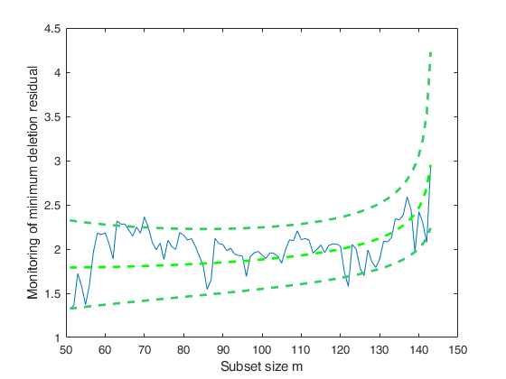
Example where initial subset comes from LTSts.
Example where initial subset comes from LTSts.In this example the units forming subset are stored just for selected steps.
%   1949 1950 1951 1952 1953 1954 1955 1956 1957 1958 1959 1960
y = [112  115  145  171  196  204  242  284  315  340  360  417    % Jan
118  126  150  180  196  188  233  277  301  318  342  391    % Feb
132  141  178  193  236  235  267  317  356  362  406  419    % Mar
129  135  163  181  235  227  269  313  348  348  396  461    % Apr
121  125  172  183  229  234  270  318  355  363  420  472    % May
135  149  178  218  243  264  315  374  422  435  472  535    % Jun
148  170  199  230  264  302  364  413  465  491  548  622    % Jul
148  170  199  242  272  293  347  405  467  505  559  606    % Aug
136  158  184  209  237  259  312  355  404  404  463  508    % Sep
119  133  162  191  211  229  274  306  347  359  407  461    % Oct
104  114  146  172  180  203  237  271  305  310  362  390    % Nov
118  140  166  194  201  229  278  306  336  337  405  432 ]; % Dec
y=(y(:));
% Set up the model.
model=struct;
model.trend=1;              % linear trend
model.s=12;                 % monthly time series
model.seasonal=104;         % four harmonics with time varying seasonality
% Call LTSts
out=LTSts(y,'model',model');
% Extract best initial subset from LTSts.
[~,indres]=sort(abs(out.residuals));
bs=indres(1:50);
[mdr,Un,BB,Bols,S2,Exflag] =FSRtsmdr(y,bs,'model',model,'init',length(bs)+1,'plots',1);
Input Arguments
Output Arguments
References
Atkinson, A.C. and Riani, M. (2006), Distribution theory and simulations for tests of outliers in regression, "Journal of Computational and Graphical Statistics", Vol. 15, pp. 460-476.
Riani, M. and Atkinson, A.C. (2007), Fast calibrations of the forward search for testing multiple outliers in regression, "Advances in Data Analysis and Classification", Vol. 1, pp. 123-141.
Rousseeuw, P.J., Perrotta D., Riani M. and Hubert, M. (2018), Robust Monitoring of Many Time Series with Application to Fraud Detection, "Econometrics and Statistics". [RPRH]