FSRts
FSRts is an automatic adaptive procedure to detect outliers in time series
Description
Examples
FSRts with all default options.
Reset the random generator
rng('default')
n=200;
rng(123456);
outSIM=simulateTS(n,'plots',1);
% Uncontaminated data
y=outSIM.y;
% FSRts and LTSts on Uncontaminated data (conflev defaults differ)
[outFSRu] = FSRts(y,'plots',1);
[outLTSu] = LTSts(y,'plots',1,'conflev',0.99);
outFSRu.outliers
outLTSu.outliers'
% Contaminated data
close all
ycont=y;
ycont(10:15) = ycont(10:15)+2*mean(ycont)*sign(ycont(10:15));
% FSRts and LTSts on contaminated data (conflev defaults differ)
[outFSR] = FSRts(ycont,'plots',1);
[outLTS] = LTSts(ycont,'plots',1,'conflev',0.99);
outFSR.outliers
outLTS.outliers'
 FSRts with optional arguments.
 FSRts with optional arguments.
rng(1)
model=struct;
model.trend=[];
model.trendb=[];
model.seasonal=103;
model.seasonalb=40*[0.1 -0.5 0.2 -0.3 0.3 -0.1 0.222];
model.signal2noiseratio=20;
T=100;
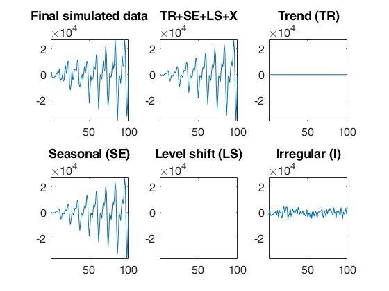
outSIM=simulateTS(T,'model',model,'plots',1);
y=outSIM.y;
model1=struct;
model1.trend=1;              % linear trend
model1.s=12;                 % monthly time series
model1.lshift=0;             % No level shift
model1.seasonal=104;         % Four harmonics
out=FSRts(y,'model',model1);
-------------------------
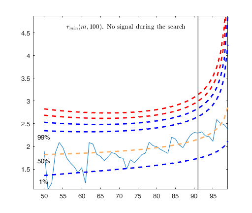
Signal detection loop
Sample seems homogeneous, no outlier has been found
Summary of the exceedances
           1          99         999        9999       99999
           4           0           0           0           0


ans =

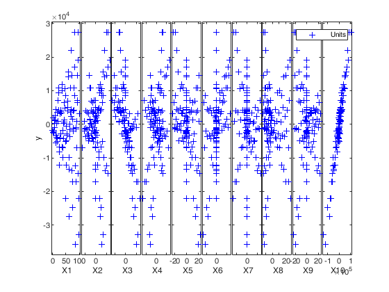
  Legend ( Units) with properties:

         String: {' Units'}
       Location: 'northeast'
    Orientation: 'vertical'
       FontSize: 7.2000
       Position: [0.8160 0.8622 0.0795 0.0371]
          Units: 'normalized'

  Use GET to show all properties
Related Examples
FSRts with optional arguments in time series with outliers.
A time series of 100 observations is simulated from a model which contains no trend, a linear time varying seasonal component with three harmonics, no explanatory variables and a signal to noise ratio equal to 20.
rng(1)
model=struct;
model.trend=[];
model.trendb=[];
model.seasonal=103;
model.seasonalb=40*[0.1 -0.5 0.2 -0.3 0.3 -0.1 0.222];
model.signal2noiseratio=20;
T=100;
outSIM=simulateTS(T,'model',model,'plots',1);
y=outSIM.y;
y(80:90)=y(80:90)+15000;
model1=struct;
model1.trend=1;              % linear trend
model1.s=12;                 % monthly time series
model1.lshift=0;
model1.seasonal=104;
out=FSRts(y,'model',model1);
 Example of the use of option lms as a vector.
 Example of the use of option lms as a vector.
A time series of 100 observations is simulated from a model which contains no trend, a linear time varying seasonal component with three harmonics, no explanatory variables and a signal to noise ratio equal to 20
rng(1)
model=struct;
model.trend=[];
model.trendb=[];
model.seasonal=103;
model.seasonalb=40*[0.1 -0.5 0.2 -0.3 0.3 -0.1 0.222];
model.signal2noiseratio=20;
T=100;
outSIM=simulateTS(T,'model',model);
y=outSIM.y;
% Contaminate the series.
y(80:90)=y(80:90)+15000;
model1=struct;
model1.trend=1;              % linear trend
model1.s=12;                 % monthly time series
model1.seasonal=104;
% Initialize the search with the first 20 units.
out=FSRts(y,'model',model1,'lms',1:20);
-------------------------
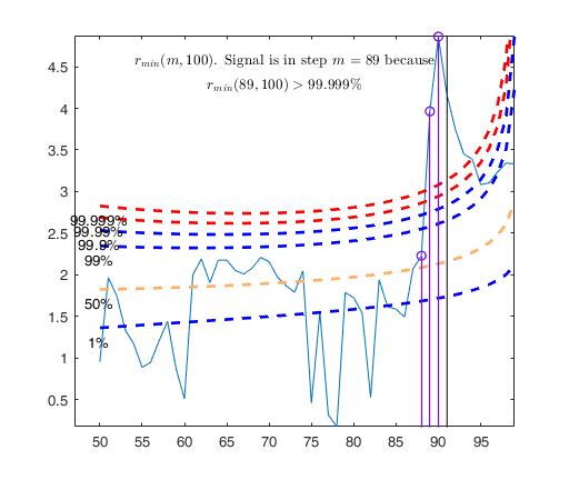
Signal detection loop
Tentative signal in central part of the search: step m=89 because
rmin(89,100)>99.999%

-------------------
Signal validation exceedance of upper envelopes
Validated signal
-------------------------------
Start resuperimposing envelopes from step m=88
Superimposition stopped because r_{min}(89,91)>99% envelope
$r_{min}(89,91)>99$\% envelope
Subsample of 90 units is homogeneous
----------------------------
Final output
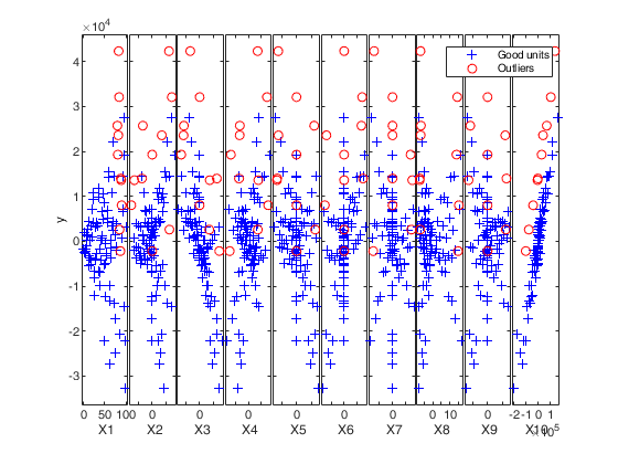
Number of units declared as outliers=10
Summary of the exceedances
           1          99         999        9999       99999
          16           9           6           6           5

 Example of the use of option lms as struct.
 Example of the use of option lms as struct.
A time series of 100 observations is simulated from a model which contains no trend, a linear time varying seasonal component with three harmonics, no explanatory variables and a signal to noise ratio equal to 20.
rng(1)
model=struct;
model.trend=[];
model.trendb=[];
model.seasonal=102;
model.seasonalb=40*[0.1 -0.5 0.2 0.3 0.01];
model.signal2noiseratio=20;
model.lshift=30;
model.lshiftb=2000;
T=100;
outSIM=simulateTS(T,'model',model,'plots',1);
y=outSIM.y;
% Contaminate the series.
y(80:90)=y(80:90)+2000;
model1=struct;
model1.trend=1;              % linear trend
model1.s=12;                 % monthly time series
model1.seasonal=104;
lms=struct;
lms.bsb=[1:20 80:85];
lms.posLS=30;
% Initialize the search with the units inside lms.bsb.
out=FSRts(y,'model',model1,'lms',lms);
-------------------------
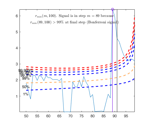
Signal detection loop
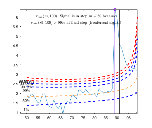
Tentative signal in central part of the search: step m=89 because
rmin(89,100)>99.999%
rmin(89,100)>99% at final step: Bonferroni signal in the central part of the search.

-------------------
Signal validation exceedance of upper envelopes
Validated signal
-------------------------------
Start resuperimposing envelopes from step m=88
Superimposition stopped because r_{min}(89,90)>99% envelope
$r_{min}(89,90)>99$\% envelope
----------------------------
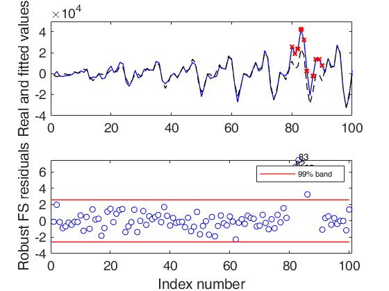
Final output
Number of units declared as outliers=11
Summary of the exceedances
           1          99         999        9999       99999
          16           9           7           7           6

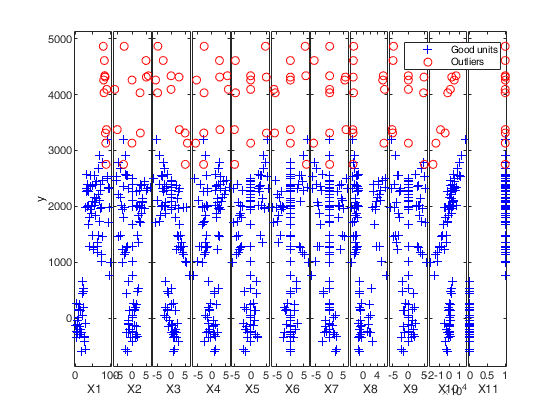
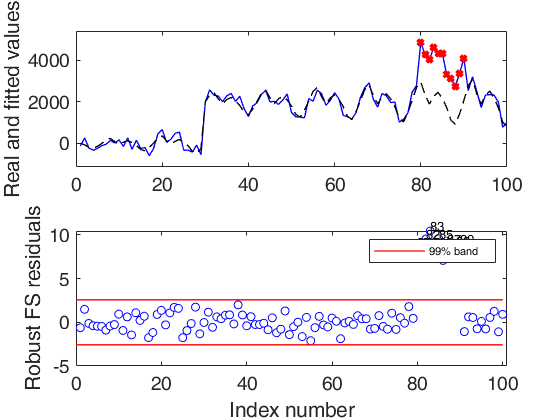
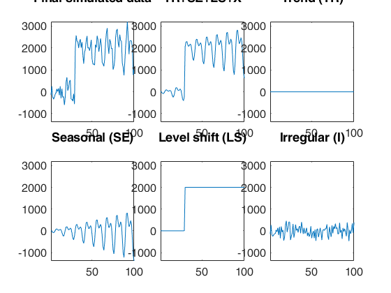
 Automatic outlier and level shift detection.
 Automatic outlier and level shift detection.
A time series of 100 observations is simulated from a model which contains no trend, a linear time varying seasonal component with three harmonics, no explanatory variables and a signal to noise ratio equal to 20.
rng(1)
model=struct;
model.trend=[];
model.trendb=[];
model.seasonal=102;
model.seasonalb=40*[0.1 -0.5 0.2 0.3 0.01];
model.signal2noiseratio=20;
model.lshift=30;
model.lshiftb=2000;
T=100;
outSIM=simulateTS(T,'model',model,'plots',1);
y=outSIM.y;
% Contaminate the series.
y(80:90)=y(80:90)+2000;
model1=struct;
model1.trend=1;              % linear trend
model1.s=12;                 % monthly time series
model1.seasonal=104;
model1.lshift=-1;
% Automatically search for outliers and level shift
out=FSRts(y,'model',model1,'msg',0);

Input Arguments
y — Time series to analyze.
Vector.
A row or a column vector with T elements, which contains the time series.
Data Types: single| double
Name-Value Pair Arguments
Specify optional comma-separated pairs of Name,Value arguments.
Name is the argument name and Value
is the corresponding value. Name must appear
inside single quotes (' ').
You can specify several name and value pair arguments in any order as
Name1,Value1,...,NameN,ValueN.
 'model', model
, 'nsamp',1000
, 'lms',1
, 'h',round(n*0.55)
, 'plots',1
, 'init',100 starts monitoring from step m=100
, 'nocheck',true
, 'bivarfit','2'
, 'multivarfit','1'
, 'labeladd','1'
, 'nameX',{'NameVar1','NameVar2'}
, 'namey','NameOfResponse'
, 'bonflev',0.99
, 'msg',1
, 'bsbmfullrank',1
, 'tag',{'plmdr' 'plyXplot'};
model
—Model type.structure.
A structure which specifies the model which will be used. The model structure contains the following fields:
| Value | Description |
|---|---|
s |
scalar (length of seasonal period). For monthly data s=12 (default), for quarterly data s=4, ... |
trend |
scalar (order of the trend component). trend = 1 implies linear trend with intercept (default), trend = 2 implies quadratic trend and so on. Admissible values for trend are, 0, 1, 2 and 3. |
seasonal |
scalar (integer specifying number of frequencies, i.e. harmonics, in the seasonal component. Possible values for seasonal are , where [s/2]=floor(s/2). For example: if seasonal =1 (default) we have: \beta_1 \cos( 2 \pi t/s) + \beta_2 sin ( 2 \pi t/s); if seasonal =2 we have: \beta_1 \cos( 2 \pi t/s) + \beta_2 \sin ( 2 \pi t/s) + \beta_3 \cos(4 \pi t/s) + \beta_4 \sin (4 \pi t/s). Note that when s is even, the sine term disappears for j=s/2 and so the maximum number of trigonometric parameters is s-1. If seasonal is a number greater than 100, then it is possible to specify how the seasonal component grows over time. For example, seasonal =101 implies a seasonal component which just uses one frequency, which grows linearly over time as follows: (1+\beta_3 t)\times ( \beta_1 cos( 2 \pi t/s) + \beta_2 \sin ( 2 \pi t/s)). For example, seasonal =201 implies a seasonal component which just uses one frequency, which grows in a quadratic way over time as follows: (1+\beta_3 t + \beta_4 t^2)\times( \beta_1 \cos( 2 \pi t/s) + \beta_2 \sin ( 2 \pi t/s)). seasonal =0 implies a non seasonal model. |
X |
matrix of size T-by-nexpl containing the values of nexpl extra covariates which are likely to affect y. |
posLS |
positive integer which specifies the position to include the level shift component. For example, if model.posLS =13, then the explanatory variable I(t \geq 13}) is created. If this field is not present or if it is empty, the level shift component is not included. |
B |
column vector or matrix containing the initial values of parameter estimates which have to be used in the maximization procedure. If model.B is a matrix, then initial estimates are extracted from the first column of this matrix. If this field is empty or if this field is not present, the initial values to be used in the maximization procedure are referred to the OLS parameter estimates of the linear part of the model. The parameters associated to time varying amplitude are initially set to 0. Remark: the default model is for monthly data with a linear trend (2 parameters) + seasonal component with just one harmonic (2 parameters), no additional explanatory variables and no level shift that is model=struct; model.s=12; model.trend=1; model.seasonal=1; model.X=''; model.posLS=''; |
Example: 'model', model
Data Types: struct
nsamp
—Number of subsamples which will be extracted to find the
robust estimator.scalar.
If nsamp=0 all subsets will be extracted.
They will be (n choose p).
If the number of all possible subset is <1000, the default is to extract all subsets otherwise just 1000.
Example: 'nsamp',1000
Data Types: double
lms
—Criterion to use to find the initial subset to initialize
the search.scalar, vector | structure.
lms specifies the criterion to use to find the initial subset to initialize the search (LTS with concentration steps or subset supplied directly by the user).
The default value is 1 (Least trimmed squares is computed to initialize the search).
If lms is a struct, it is possible to control a series of options for concentration steps (for more details see function LTSts.m) If, on the other hand, the user wants to initialize the search with a prespecified set of units, there are two possibilities: 1) lms can be a vector with length greater than 1 which contains the list of units forming the initial subset. For example, if the user wants to initialize the search with units 4, 6 and 10 then lms=[4 6 10];
2) lms is a struct which contains a field named bsb which contains the list of units to initialize the search. For example, in the case of simple regression through the origin with just one explanatory variable, if the user wants to initialize the search with unit 3 then lms=struct;
| Value | Description |
|---|---|
bsb |
3; |
Example: 'lms',1
Data Types: double
h
—The number of observations that have determined the least
trimmed squares estimator.scalar.
h is an integer greater or equal than p, but smaller then n. Generally, if the purpose is outlier detection h=[0.5*(n+p+1)] (default value). h can be smaller than this threshold if the purpose is to find subgroups of homogeneous observations.
In this function the LTSts estimator is used just to initialize the search. The default value of h which is used is round(0.75*T).
Example: 'h',round(n*0.55)
Data Types: double
plots
—Plot on the screen.scalar.
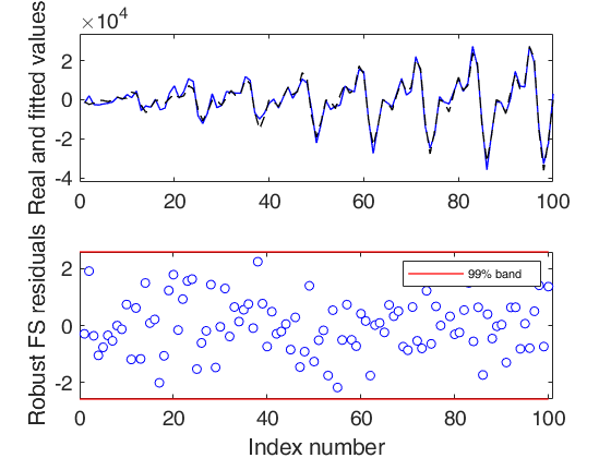
If plots=1 (default), the plot of minimum deletion residual with envelopes based on T observations and the scatterplot matrix with the outliers highlighted is produced together with a two panel plot.
The upper panel contains the original time series with fitted values. The bottom panel will contain the plot of robust residuals against index number. The confidence level, which is used to draw the horizontal lines associated with the bands for the residuals, is 0.999.
If plots=2, the user can also monitor the intermediate plots based on envelope superimposition.
Else no plot is produced.
Example: 'plots',1
Data Types: double
init
—Start of monitoring point.scalar.
It specifies the point where to initialize the search and start monitoring required diagnostics. If it is not specified, it is set equal floor(0.5*(T+1)).
Example: 'init',100 starts monitoring from step m=100
Data Types: double
nocheck
—Check input arguments inside input option model.as default nocheck=false.
Example: 'nocheck',true
Data Types: boolean
bivarfit
—Superimpose bivariate least square lines.character.
This option adds one or more least squares lines, based on SIMPLE REGRESSION of y on Xi, to the plots of y|Xi.
bivarfit = '' is the default: no line is fitted.
bivarfit = '1' fits a single ols line to all points of each bivariate plot in the scatter matrix y|X.
bivarfit = '2' fits two ols lines: one to all points and another to the group of the genuine observations. The group of the potential outliers is not fitted.
bivarfit = '0' fits one ols line to each group. This is useful for the purpose of fitting mixtures of regression lines.
bivarfit = 'i1' or 'i2' or 'i3' etc. fits an ols line to a specific group, the one with index 'i' equal to 1, 2, 3 etc. Again, useful in case of mixtures.
Example: 'bivarfit','2'
Data Types: char
multivarfit
—Superimpose multivariate least square lines.character.
This option adds one or more least square lines, based on MULTIVARIATE REGRESSION of y on X, to the plots of y|Xi.
multivarfit = '' is the default: no line is fitted.
multivarfit = '1' fits a single ols line to all points of each bivariate plot in the scatter matrix y|X. The line added to the scatter plot y|Xi is avconst + Ci*Xi, where Ci is the coefficient of Xi in the multivariate regression and avconst is the effect of all the other explanatory variables different from Xi evaluated at their centroid (that is overline{y}'C)).
multivarfit = '2' equal to multivarfit ='1', but this time we also add the line based on the group of unselected observations (i.e. the normal units).
Example: 'multivarfit','1'
Data Types: char
labeladd
—Add outlier labels in plot.character.
If this option is '1', we label the outliers with the unit row index in matrices X and y. The default value is labeladd='', i.e. no label is added.
Example: 'labeladd','1'
Data Types: char
nameX
—Add variable labels in plot.cell array of strings.
Cell array of strings of length p containing the labels of the variables of the regression dataset. If it is empty (default) the sequence X1, ..., Xp will be created automatically
Example: 'nameX',{'NameVar1','NameVar2'}
Data Types: cell
namey
—Add response label.character.
String containing the label of the response
Example: 'namey','NameOfResponse'
Data Types: char
ylim
—Control y scale in plot.vector.
Vector with two elements controlling minimum and maximum on the y axis.
Default value is '' (automatic scale)
Example: 'ylim',[0,10] sets the minimum value to 0 and the
max to 10 on the y axis
Data Types: double
xlim
—Control x scale in plot.vector.
Vector with two elements minimum and maximum on the x axis. Default value is '' (automatic scale)
Example: 'xlim',[0,10] sets the minimum value to 0 and the
max to 10 on the x axis
Data Types: double
bonflev
—Signal to use to identify outliers.scalar.
Option to be used if the distribution of the data is strongly non normal and, thus, the general signal detection rule based on consecutive exceedances cannot be used. In this case bonflev can be: - a scalar smaller than 1, which specifies the confidence level for a signal and a stopping rule based on the comparison of the minimum MD with a Bonferroni bound. For example, if bonflev=0.99 the procedure stops when the trajectory exceeds for the first time the 99% bonferroni bound.
- A scalar value greater than 1. In this case, the procedure stops when the residual trajectory exceeds for the first time this value.
Default value is '', which means to rely on general rules based on consecutive exceedances.
Example: 'bonflev',0.99
Data Types: double
msg
—Level of output to display.scalar.
It controls whether to display or not messages on the screen.
If msg==1 (default), messages are displayed on the screen about step in which signal took place, else no message is displayed on the screen.
Example: 'msg',1
Data Types: double
bsbmfullrank
—Dealing with singular X matrix.scalar.
This option tells how to behave in case subset at step m (say bsbm) produces a singular X. In other words, this options controls what to do when rank(X(bsbm,:)) is smaller than number of explanatory variables. If bsbmfullrank =1 (default), these units (whose number is say mnofullrank) are constrained to enter the search in the final n-mnofullrank steps, else the search continues using as estimate of beta at step m the estimate of beta found in the previous step.
Example: 'bsbmfullrank',1
Data Types: double
tag
—tags to the plots which are created.character | cell array of characters.
This option enables to add a tag to the plots which are created. The default tag names are: fsr_mdrplot for the plot of mdr based on all the observations;
fsr_yXplot for the plot of y against each column of X with the outliers highlighted;
fsr_resuperplot for the plot of resuperimposed envelopes. The first plot with 4 panel of resuperimposed envelopes has tag fsr_resuperplot1, the second fsr_resuperplot2 ...
If tag is a character or a cell of characters of length 1, it is possible to specify the tag for the plot of mdr based on all the observations;
If tag is a cell of length 2 it is possible to control both the tag for the plot of mdr based on all the observations and the tag for the yXplot with outliers highlighted.
If tag is a cell of length 3 the third element specifies the names of the plots of resuperimposed envelopes.
Example: 'tag',{'plmdr' 'plyXplot'};
Data Types: char or cell
Output Arguments
out — description
Structure
Structure which contains the following fields
| Value | Description |
|---|---|
ListOut |
k x 1 vector containing the list of the units declared as outliers or NaN if the sample is homogeneous. |
outliers |
out.ListOut. This field is added for homogeneity with the other robust estimators. |
beta |
Matrix containing estimated beta coefficients, standard errors, t-stat and p-values. The content of matrix out.beta is as follows: 1st col = beta coefficients The order of the beta coefficients is as follows: 1) trend elements (if present). If the trend is of order two, there are r+1 coefficients if the intercept is present; otherwise, there are just r components; 2) linear part of seasonal component 2, 4, 6, ..., s-2, s-1 coefficients (if present); 3) coefficients associated with the matrix of explanatory variables which have a potential effect on the time series under study (X); 4) non linear part of seasonal component, that is varying amplitude. If varying amplitude is of order k, there are k coefficients (if present); 5) level shift component (if present). In this case, there are two coefficients, the second (which is also the last element of vector beta) is an integer, which specifies the time in which level shift takes place and the first (which is also the penultimate element of vector beta) is a real number which identifies the magnitude of the upward (downward) level shift; 2nd col = standard errors; 3rd col = t-statistics; 4th col = p values. |
scale |
scalar containing the estimate of the scale (sigma). |
residuals |
n x 1 vector containing the estimates of the robust scaled residuals. |
fittedvalues |
n x 1 vector containing the fitted values. |
mdr |
(n-init) x 2 matrix 1st col = fwd search index 2nd col = value of minimum deletion residual in each step of the fwd search Exflag : Reason nlinfit stopped. Integer matrix. (n-init+1) x 2 matrix containing information about the result of the maximization procedure. If the model is non linear, out.Exflag(i,2) is equal to 1 if at step out.Exflag(i,1) the maximization procedure did not produce warnings or the warning was different from "ILL Conditioned Jacobian". For any other warning that is produced (for example, "Overparameterized", "IterationLimitExceeded", 'MATLAB:rankDeficientMatrix") out.Exflag(i,2) is equal to -1; |
Un |
(n-init) x 11 matrix which contains the unit(s) included in the subset at each step of the fwd search. REMARK: in every step the new subset is compared with the old subset. Un contains the unit(s) present in the new subset but not in the old one. Un(1,2), for example, contains the unit included in step init+1. Un(end,2) contains the units included in the final step of the search. |
nout |
2 x 5 matrix containing the number of times mdr went out of particular quantiles. First row contains quantiles 1 99 99.9 99.99 99.999. Second row contains the frequency distribution. |
constr |
This output is produced only if the search found at a certain step X is a singular matrix. In this case, the search runs in a constrained mode, that is including the units which produced a non singular matrix in the last n-constr steps. out.constr is a vector which contains the list of units which produced a singular X matrix |
Exflag |
Reason nlinfit stopped. Integer matrix. (n-init+1) x 2 matrix containing information about the result of the maximization procedure. If the model is non linear, out.Exflag(i,2) is equal to 1; if at step out.Exflag(i,1) the maximization procedure did not produce warnings or the warning was different from "ILL Conditioned Jacobian". For any other warning which is produced (for example, "Overparameterized", "IterationLimitExceeded", 'MATLAB:rankDeficientMatrix") out.Exflag(i,2) is equal to -1; |
class |
'FSRts'. |
References
Riani, M., Atkinson, A.C. and Cerioli, A. (2009), Finding an unknown number of multivariate outliers, "Journal of the Royal Statistical Society Series B", Vol. 71, pp. 201-221.
Rousseeuw, P.J., Perrotta D., Riani M. and Hubert, M. (2018), Robust Monitoring of Many Time Series with Application to Fraud Detection, "Econometrics and Statistics". [RPRH]