FSRts
FSRts is an automatic adaptive procedure to detect outliers in time series
Description
Examples
 FSRts with optional arguments.
FSRts with optional arguments.
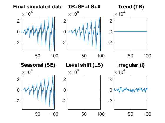
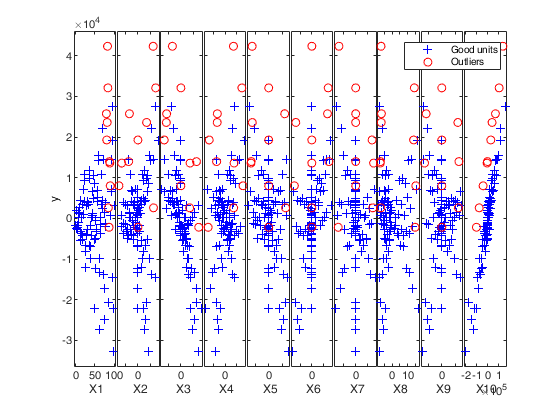
rng(1)
model=struct;
model.trend=[];
model.trendb=[];
model.seasonal=103;
model.seasonalb=40*[0.1 -0.5 0.2 -0.3 0.3 -0.1 0.222];
model.signal2noiseratio=20;
T=100;
outSIM=simulateTS(T,'model',model,'plots',1);
y=outSIM.y;
model1=struct;
model1.trend=1;              % linear trend
model1.s=12;                 % monthly time series
model1.lshift=0;             % No level shift
model1.seasonal=104;         % Four harmonics
out=FSRts(y,'model',model1);
-------------------------
Signal detection loop
Sample seems homogeneous, no outlier has been found
Summary of the exceedances
           1          99         999        9999       99999
           4           0           0           0           0

Related Examples
Example of the use of option lms as a vector.
Example of the use of option lms as a vector.A time series of 100 observations is simulated from a model which contains no trend, a linear time varying seasonal component with three harmonics, no explanatory variables and a signal to noise ratio equal to 20
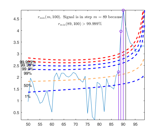
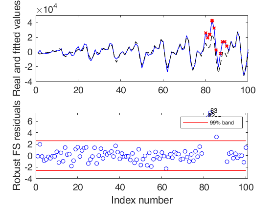
rng(1)
model=struct;
model.trend=[];
model.trendb=[];
model.seasonal=103;
model.seasonalb=40*[0.1 -0.5 0.2 -0.3 0.3 -0.1 0.222];
model.signal2noiseratio=20;
T=100;
outSIM=simulateTS(T,'model',model);
y=outSIM.y;
% Contaminate the series.
y(80:90)=y(80:90)+15000;
model1=struct;
model1.trend=1;              % linear trend
model1.s=12;                 % monthly time series
model1.seasonal=104;
% Initialize the search with the first 20 units.
out=FSRts(y,'model',model1,'lms',1:20);
-------------------------
Signal detection loop
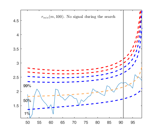
Tentative signal in central part of the search: step m=89 because
rmin(89,100)>99.999%
-------------------
Signal validation exceedance of upper envelopes
Validated signal
-------------------------------
Start resuperimposing envelopes from step m=88
Superimposition stopped because r_{min}(89,91)>99% envelope
$r_{min}(89,91)>99$\% envelope
Subsample of 90 units is homogeneous
----------------------------
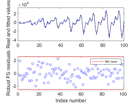
Final output
Number of units declared as outliers=10
Summary of the exceedances
1 99 999 9999 99999
16 9 6 6 5
Example of the use of option lms as struct.
Example of the use of option lms as struct.A time series of 100 observations is simulated from a model which contains no trend, a linear time varying seasonal component with three harmonics, no explanatory variables and a signal to noise ratio equal to 20.
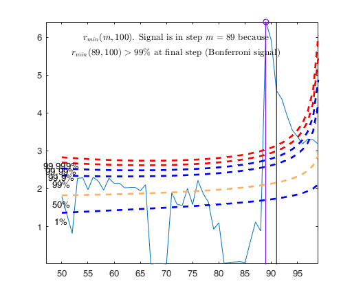
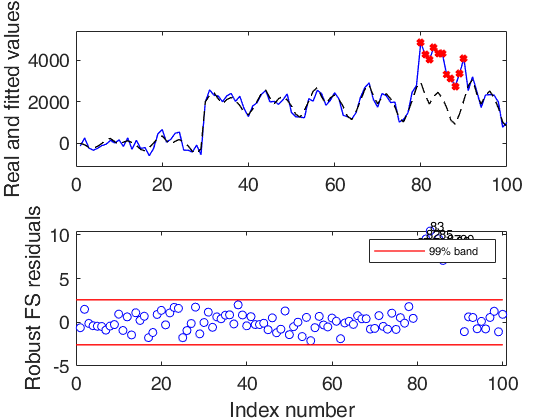
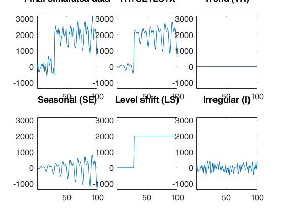
rng(1)
model=struct;
model.trend=[];
model.trendb=[];
model.seasonal=102;
model.seasonalb=40*[0.1 -0.5 0.2 0.3 0.01];
model.signal2noiseratio=20;
model.lshift=30;
model.lshiftb=2000;
T=100;
outSIM=simulateTS(T,'model',model,'plots',1);
y=outSIM.y;
% Contaminate the series.
y(80:90)=y(80:90)+2000;
model1=struct;
model1.trend=1;              % linear trend
model1.s=12;                 % monthly time series
model1.seasonal=104;
lms=struct;
lms.bsb=[1:20 80:85];
lms.posLS=30;
% Initialize the search with the units inside lms.bsb.
out=FSRts(y,'model',model1,'lms',lms);
-------------------------
Signal detection loop
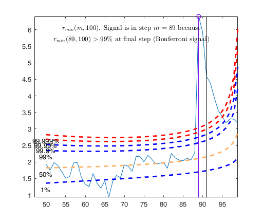
Tentative signal in central part of the search: step m=89 because
rmin(89,100)>99.999%
rmin(89,100)>99% at final step: Bonferroni signal in the central part of the search.
-------------------
Signal validation exceedance of upper envelopes
Validated signal
-------------------------------
Start resuperimposing envelopes from step m=88
Superimposition stopped because r_{min}(89,90)>99% envelope
$r_{min}(89,90)>99$\% envelope
----------------------------
Final output
Number of units declared as outliers=11
Summary of the exceedances
1 99 999 9999 99999
16 9 7 7 6

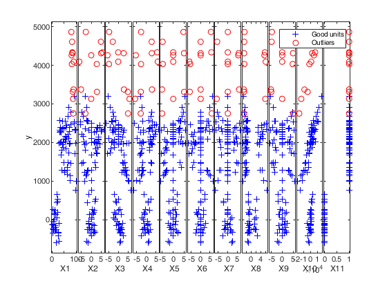
Automatic outlier and level shift detection.
Automatic outlier and level shift detection.A time series of 100 observations is simulated from a model which contains no trend, a linear time varying seasonal component with three harmonics, no explanatory variables and a signal to noise ratio equal to 20.
rng(1)
model=struct;
model.trend=[];
model.trendb=[];
model.seasonal=102;
model.seasonalb=40*[0.1 -0.5 0.2 0.3 0.01];
model.signal2noiseratio=20;
model.lshift=30;
model.lshiftb=2000;
T=100;
outSIM=simulateTS(T,'model',model,'plots',1);
y=outSIM.y;
% Contaminate the series.
y(80:90)=y(80:90)+2000;
model1=struct;
model1.trend=1;              % linear trend
model1.s=12;                 % monthly time series
model1.seasonal=104;
model1.lshift=-1;
% Automatically search for outliers and level shift
out=FSRts(y,'model',model1,'msg',0);

Input Arguments
Output Arguments
References
Riani, M., Atkinson, A.C. and Cerioli, A. (2009), Finding an unknown number of multivariate outliers, "Journal of the Royal Statistical Society Series B", Vol. 71, pp. 201-221.
Rousseeuw, P.J., Perrotta D., Riani M. and Hubert, M. (2018), Robust Monitoring of Many Time Series with Application to Fraud Detection, "Econometrics and Statistics". [RPRH]