FSRr
Forward search in linear regression reweighted
Description
FSRr uses the units not declared by outliers by FSR to produce a robust fit.
The units whose residuals exceeds the threshold determined by option alpha are declared as outliers. Moreover, it is possible in option R2th to modify the estimate of sigma2 which is used to declare the outliers. This is useful when there is almost a perfect fit in the data, the estimate of the error variance is very small and therefore there is the risk of declaring as outliers very small deviations from the robust fit. In this case, the estimate of sigma2 is corrected in order to achieve a value of R2 equal to R2th.
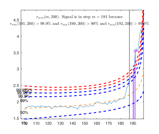
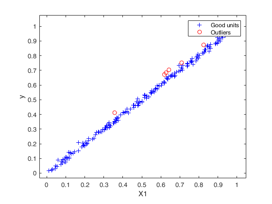
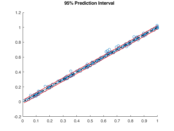
Example of outlier detection in a case of almost perfect fit.out
=FSRr(y,
X,
Name, Value)
Examples
 Example of outlier detection in a case of almost perfect fit: all default options.
Example of outlier detection in a case of almost perfect fit: all default options.
n=200; p=1;
X = rand(n,p);
y = X + 0.01*randn(n,1);
% contaminated data points
ycont = y;
ycont(1:8) = ycont(1:8)+0.05;
[out , xnew1 , ypred1, yci1] = ...
FSRr(ycont,X,'plotsPI',1,'plots',1);
disp(['Outliers without R2 adjustment = ' num2str(out.outliers)]);
disp(['Outliers with    R2 adjustment = ' num2str(out.outliersr)]);
Outliers without R2 adjustment = 1  2  4  5  6  7
Outliers with    R2 adjustment = 1    2    3    4    5    6    7    8   52   72  100  101  149  161  175
Related Examples
Input Arguments
Output Arguments
References
Riani, M., Atkinson, A.C. and Cerioli, A. (2009), Finding an unknown number of multivariate outliers, "Journal of the Royal Statistical Society Series B", Vol. 71, pp. 201-221.