
|
MMmult |
MMmulteda |
 |
MMmultcore
MMmultcore computes multivariate MM estimators for a selected fixed scale
Syntax
Description
Examples
 MMmultcore with optional arguments.
MMmultcore with optional arguments.Determine, e.g., an S estimate and extract the required arguments for the MM estimate.
n=200;
v=3;
randn('state', 123456);
Y=randn(n,v);
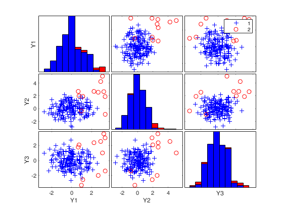
% Contaminated data
Ycont=Y;
Ycont(1:5,:)=Ycont(1:5,:)+3;
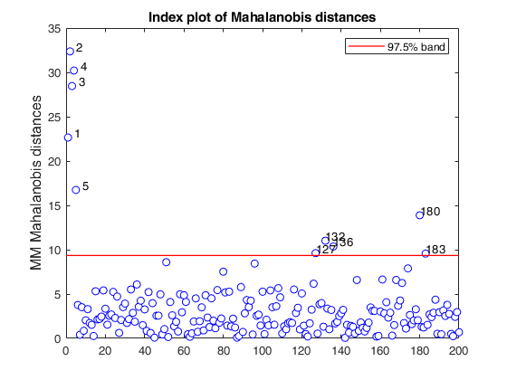
[outS]=Smult(Ycont,'plots',1);
out=MMmultcore(Ycont,outS.loc,outS.shape,outS.scale,'plots',1,'nocheck',1);
Warning: Using 'state' to set RANDN's internal state causes RAND, RANDI, and
RANDN to use legacy random number generators.  This syntax is not recommended.
See <a href="matlab:helpview([docroot '\techdoc\math\math.map'],'update_random_number_generator')">Replace Discouraged Syntaxes of rand and randn</a> to use RNG to replace the
old syntax.
Total estimated time to complete S estimator:  0.48 seconds


Input Arguments
Output Arguments
More About
References
Maronna, R.A., Martin D. and Yohai V.J. (2006), "Robust Statistics, Theory and Methods", Wiley, New York.
Acknowledgements
This function follows the lines of MATLAB/R code developed during the years by many authors. For more details see the R library robustbase http://robustbase.r-forge.r-project.org/.
The core of these routines, e.g. the resampling approach, however, has been completely redesigned, with considerable increase of the computational performance.