SDest
SDest computes Stahel-Donoho robust estimator of dispersion-location
Description
Examples
 SDest with optional arguments.
SDest with optional arguments.SDest with v+1 directions for each subsample (jpcorr=1).
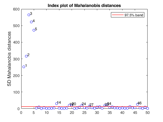
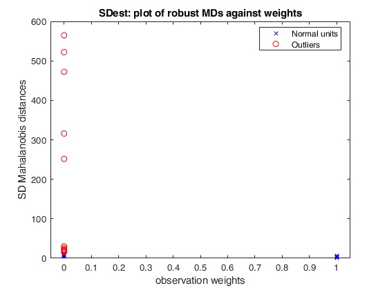
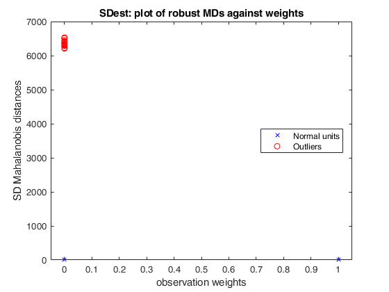
% Produce plot of robust Mahalanobis distances
n=50;
v=5;
randn('state', 1256);
Y=randn(n,v);
% Contaminated data
Ycont=Y;
Ycont(1:5,:)=Ycont(1:5,:)+4;
[out]=SDest(Ycont,'jpcorr',1,'plots',1);
Warning: Using 'state' to set RANDN's internal state causes RAND, RANDI, and
RANDN to use legacy random number generators.  This syntax is not recommended.
See <a href="matlab:helpview([docroot '\techdoc\math\math.map'],'update_random_number_generator')">Replace Discouraged Syntaxes of rand and randn</a> to use RNG to replace the
old syntax.
Total estimated time to complete Stahel-Donoho estimator:  0.24 seconds

Related Examples
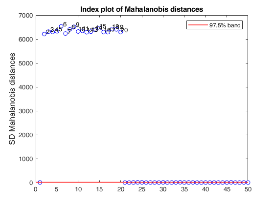
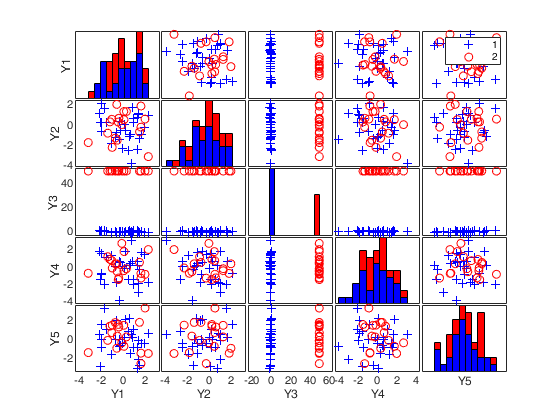
SDest jpcorr equal to 1.
SDest jpcorr equal to 1.v+1 directions for each subsample. Produce plot of robust Mahalanobis distances.
n=50;
v=5;
randn('state', 1256);
Y=randn(n,v);
% Contaminated data
Ycont=Y;
Ycont(2:20,3)=100;
[out]=SDest(Ycont,'jpcorr',1,'margin',3,'plots',1);
Total estimated time to complete Stahel-Donoho estimator:  0.19 seconds
Warning: Matrix is singular to working precision.
Warning: Matrix is singular to working precision.
Warning: Matrix is singular to working precision.
Warning: Matrix is singular to working precision.
Warning: Matrix is singular to working precision.
Warning: Matrix is singular to working precision.
Warning: Matrix is singular to working precision.
Warning: Matrix is singular to working precision.
Warning: Matrix is singular to working precision.
Warning: Matrix is singular to working precision.
Warning: Matrix is singular to working precision.
Warning: Matrix is singular to working precision.
Warning: Matrix is singular to working precision.
Warning: Matrix is singular to working precision.
Warning: Matrix is singular to working precision.
Warning: Matrix is singular to working precision.
Warning: Matrix is singular to working precision.
Warning: Matrix is singular to working precision.
Warning: Matrix is singular to working precision.
Warning: Matrix is singular to working precision.
Warning: Matrix is singular to working precision.
Warning: Matrix is singular to working precision.
Input Arguments
Output Arguments
More About
References
Stahel, W.A. (1981), "Breakdown of covariance estimators", Research Report 31, Fachgruppe for Statistik, E.T.H. Zurich, Switzerland.
Donoho, D.L. (1982), "Breakdown Properties of Multivariate Location Estimators", Ph.D. dissertation, Harvard University.
Maronna, R.A. and Yohai, V.J. (1995), The behavior of the Stahel-Donoho robust multivariate estimator, "Journal of the American Statistical Association", Vol. 90, pp. 329-341.
Juan J. and Prieto F.J. (1995), "Journal of Computational and Graphical Statistics", Vol. 4, pp. 319-334.
Maronna, R.A., Martin D. and Yohai V.J. (2006), Robust Statistics, Theory and Methods, Wiley, New York.
Acknowledgements
This function follows the lines of MATLAB code developed during the years by many authors.