add2yX
add2yX adds objects (personalized clickable multilegends and text labels) to the yXplot
Description
Examples
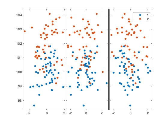
 add2yX with all default options.
add2yX with all default options.
n=100;
p=3;
X=randn(n,p);
y=100+randn(n,1);
sel=51:100;
y(sel)=y(sel)+2;
group=ones(n,1);
group(sel)=2;
[H,AX,BigAx] = gplotmatrix(X,y,group);
% The legengs are not clickable
add2yX(H,AX,BigAx)
% Now the legends become clickable
% As an alternative it was enough to use
% clickableMultiLegend
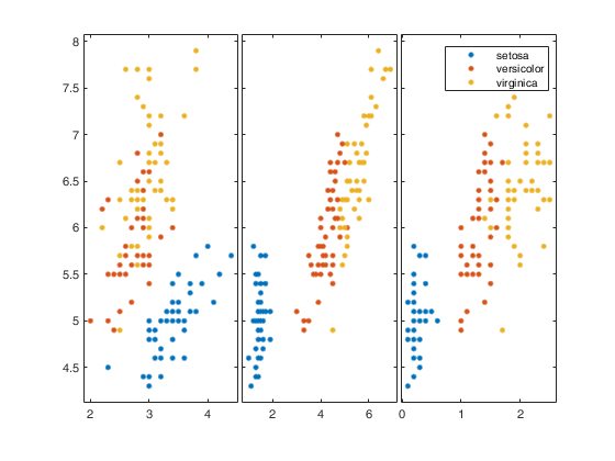
Compare gplotmatrix and addyX with yXplot for IRIS data.
Compare gplotmatrix and addyX with yXplot for IRIS data.
load fisheriris;
% Create scatter plot matrix with specific legends
% plot Sepal length (y) againt the other variables
y=meas(:,1);
X=meas(:,2:4);
[H,AX,BigAx]=gplotmatrix(X,y,species,[],[],[],'on');
% The legends are not clickable
add2yX(H,AX,BigAx)
% Now the legends become clickable
% It is easier to call directly function yXplot
[H,AX,BigAx]=yXplot(meas(:,1),meas(:,2:4),species);
Related Examples
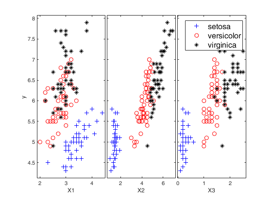
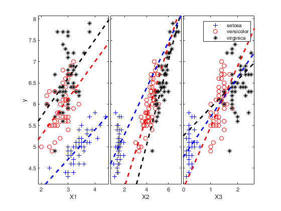
Example of use of option bivarfit.
Example of use of option bivarfit.
load fisheriris;
% Create scatter plot matrix with specific legends
% plot Sepal length (y) againt the other variables
y=meas(:,1);
X=meas(:,2:4);
[H,AX,BigAx]=yXplot(meas(:,1),meas(:,2:4),species);
% add a regression line to each group
add2yX(H,AX,BigAx,'bivarfit','0')
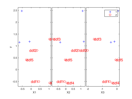
Example of use of option 'labeladd' combined with 'RowNamesLabels'.
Example of use of option 'labeladd' combined with 'RowNamesLabels'.
close all;
n=8;
y = randn(n,1);
X = randn(n,3);
group = ones(n,1);
group(1:5) = 2;
[H,AX,BigAx] = yXplot(y,X,group);
% Create cell containing the name of the rows.
label={'ddf1' 'ddf2' 'ddf3' 'ddf4' 'ddf5' 'ddf6' 'ddf7' 'ddf8'};
% Labels are added to the units which belong to group 2 (that is to the
% first 5 units). The labels are taken from cell label
add2yX(H,AX,BigAx,'labeladd','1','RowNamesLabels',label);
Input Arguments
Output Arguments
More About
References
Tufte E.R. (1983), "The visual display of quantitative information", Graphics Press, Cheshire.