yXplot
yXplot produces an interactive scatterplot of y against each variable of X in the input dataset.
Syntax
Description
Examples
yXplot with first argument vector y and no option.
In the first example as input there are two matrices y and X respectively A simple yX plot is created
n=100;
p=3;
X=randn(n,p);
y=100+randn(n,1);
% Example of the use of function yXplot with all the default options
yXplot(y,X);
yXplot with first argument vector y and third argument group.
Different groups are shown in the yXplot
n=100;
p=3;
X=randn(n,p);
y=100+randn(n,1);
sel=51:100;
y(sel)=y(sel)+2;
group=ones(n,1);
group(sel)=2;
yXplot(y,X,group);
yXplot with first argument vector y, third argument group and fourth argument plo (Ex1).
In this case plo is a scalar
n=100;
p=3;
X=randn(n,p);
y=100+randn(n,1);
sel=51:100;
y(sel)=y(sel)+2;
group=ones(n,1);
group(sel)=2;
% plo is a scalar
plo=1;
yXplot(y,X,group,plo);
yXplot with first argument vector y, third argument group and fourth argument plo (Ex2).
In this case plo is a structure
n=100;
p=3;
X=randn(n,p);
y=randn(n,1);
sel=51:100;
y(sel)=y(sel)+2;
group=ones(n,1);
group(sel)=2;
% plo is a struct
plo=struct;
% Set the scale for the x axes
plo.xlimx=[-1 2];
% Set the scale for the y axis
plo.ylimy=[0 2];
% Control symbol type
plo.sym={'^';'v'};
yXplot(y,X,group,plo);
Related Examples
yXplot with first input argument a vector, varargin is name/value pairs Ex1.
Example of use of option selunit.
% Example of the use of function yXplot putting the text for the units
% which have a value of y smaller than 98 and greater than 102.
% Note that in this case selunit is a cell array.
n=100;
p=3;
X=randn(n,p);
y=randn(n,1);
sel=51:100;
y(sel)=y(sel)+2;
yXplot(y,X,'selunit',{'98' '102'});
yXplot with first input argument a vector, varargin is name/value pairs Ex2.
yXplot with personalized labelling.
% Example of the use of function yXplot putting the text for the units
% which have a value of y smaller than 1 per cent percentile and greater than
% 99 per cent percentile of y.
% Note that in this case selunit is a cell array.
n=100;
p=3;
X=randn(n,p);
y=randn(n,1);
sel=51:100;
y(sel)=y(sel)+2;
selth={num2str(prctile(y,1)) num2str(prctile(y,99))};
yXplot(y,X,'selunit',selth);
yXplot with first input argument a vector, varargin is name/value pairs Ex2.
yXplot with personalized labelling.
% In this case selunit is passed as a numeric vector and it contains
% the list of the units which have to be labelled in the yXplot.
n=100;
p=3;
X=randn(n,p);
y=randn(n,1);
sel=51:100;
y(sel)=y(sel)+2;
selth=[2 10 20];
yXplot(y,X,'selunit',selth);
 options selunit with row names.
options selunit with row names.In this case the row names are contained inside input argument plo.label
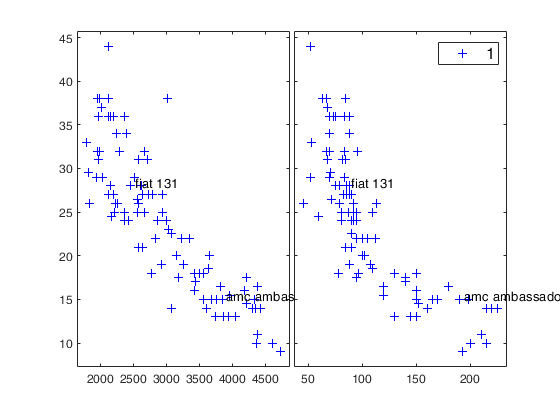
close all
load carsmall
x1 = Weight;
x2 = Horsepower;    % Contains NaN data
y = MPG;    % response
X=[x1 x2];
% Remove Nans
boo=~isnan(y);
y=y(boo,:);
X=X(boo,:);
RowLabelsMatrixY=Model(boo,:);
seluni=[10 30];
plo=struct;
plo.label=cellstr(RowLabelsMatrixY);
% add labels for units inside vector seluni
yXplot(y,X,'selunit',seluni,'plo',plo);
yXplot with first input argument a vector, varargin is name/value pairs Ex3.
n=100;
p=3;
X=randn(n,p);
y=100+randn(n,1);
sel=51:100;
y(sel)=y(sel)+2;
group=ones(n,1);
group(sel)=2;
% add a personalized tag to the figure
yXplot(y,X,'group',group,'tag','myfig');
yXplot with first input argument a vector, varargin is name/value pairs Ex4.
In this case options xlimx, ylimy, nameX and namey are used
n=100;
p=2;
X=randn(n,p);
y=100+randn(n,1);
sel=51:100;
y(sel)=y(sel)+2;
group=ones(n,1);
group(sel)=2;
% Control scale of the x axes
xlimx=[-1 4];
% Control scale of the y axis
ylimy=[99 101];
% Personalized labels for the x axes
nameX={'one' 'two'};
% Personalized labels for y axis
namey='Response';
yXplot(y,X,'group',group,'xlimx',xlimx,'ylimy',ylimy,'namey',namey,'nameX',nameX);
yXplot when first input argument y is a structure.
Ex1. In the following example the input is a strucure which also contains information about the forward search.
n=100;
p=2;
X=randn(n,p);
y=100+randn(n,1);
sel=51:100;
y(sel)=y(sel)+2;
[out]=LXS(y,X,'nsamp',1000);
[out]=FSReda(y,X,out.bs);
% Example of the use of function yXplot with all the default options
yXplot(out);
Interactive example 1.
Example of the use of options selunit and selstep.
% After the instruction below the labels for units inside vector
% selunit are added to each panel of the yXplot
n=100;
p=2;
X=randn(n,p);
y=100+randn(n,1);
sel=51:100;
y(sel)=y(sel)+2;
[out]=LXS(y,X,'nsamp',1000);
[out]=FSReda(y,X,out.bs);
selunit=[2 5 20 23 35 45];
yXplot(out,'selunit',selunit,'selstep',[20 22 27 36],...
'databrush',{'persist','off','selectionmode' 'Rect'});
%   After brushing the resfwdplot automatically appears and the labels
% are put for units contained in vector selunit in steps [20 22 27
% 36] of the search
Interactive example 2.
Example of the use of options selstep, selunit.
%   It produces a yXplot plot in which labels are put for units
%   which have a residual greater and 1.5. When a set of units is brushed in the yXplot
%   in the monitoring residuals plot the labels are added in steps
%   selsteps.
n=100;
p=2;
X=randn(n,p);
y=100+randn(n,1);
sel=51:100;
y(sel)=y(sel)+2;
[out]=LXS(y,X,'nsamp',1000);
[out]=FSReda(y,X,out.bs);
yXplot(out,'selstep',[40 21 80],'selunit','1.5',...
'databrush',{'persist','off','selectionmode' 'Rect'});
Interactive example 3.
Example of the use of option selunit (notice that in this
case selunit is a cell array of strings.
%   Highlight only the trajectories which in at least one step of the
%   search had a value smaller than -3 or greater than 2 and label
%   them at the beginning and at the end of the search.
n=100;
p=2;
X=randn(n,p);
y=100+randn(n,1);
sel=51:100;
y(sel)=y(sel)+2;
[out]=LXS(y,X,'nsamp',1000);
[out]=FSReda(y,X,out.bs);
yXplot(out,'selunit',{'-3';'2'},...
'databrush',{'selectionmode' 'Rect'});
Interactive example 4.
Example of the use of option databrush
(brushing is done only once using a rectangular selection tool).
n=100;
p=2;
X=randn(n,p);
y=100+randn(n,1);
sel=51:100;
y(sel)=y(sel)+2;
[out]=LXS(y,X,'nsamp',1000);
[out]=FSReda(y,X,out.bs);
yXplot(out,'databrush',1)
%   An equivalent statement is
yXplot(out,'databrush',{'selectionmode' 'Rect'});
Interactive example 5.
Example of the use of brush using a rectangular selection tool and
a cyan colour.
n=100;
p=2;
X=randn(n,p);
y=100+randn(n,1);
sel=51:100;
y(sel)=y(sel)+2;
[out]=LXS(y,X,'nsamp',1000);
[out]=FSReda(y,X,out.bs);
yXplot(out,'databrush',{'selectionmode' 'Rect' 'FlagColor' 'c'});
Interactive example 6.
Example of the use of brush using multiple selection circular tools.
n=100;
p=2;
X=randn(n,p);
y=100+randn(n,1);
sel=51:100;
y(sel)=y(sel)+2;
[out]=LXS(y,X,'nsamp',1000);
[out]=FSReda(y,X,out.bs);
yXplot(out,'databrush',{'selectionmode' 'Brush'});
Interactive example 7.
Example of the use of brush using lasso selection tool and fleur pointer.
n=100;
p=2;
X=randn(n,p);
y=100+randn(n,1);
sel=51:100;
y(sel)=y(sel)+2;
[out]=LXS(y,X,'nsamp',1000);
[out]=FSReda(y,X,out.bs);
yXplot(out,'databrush',{'selectionmode' 'lasso','Pointer','fleur'});
Interactive example 8.
Example of the use of rectangular brush.
Superimposed labels for the brushed units and persistent labels in the yXplot which has been brushed
n=100;
p=2;
X=randn(n,p);
y=100+randn(n,1);
sel=51:100;
y(sel)=y(sel)+2;
[out]=LXS(y,X,'nsamp',1000);
[out]=FSReda(y,X,out.bs);
yXplot(out,'databrush',{'selectionmode' 'Rect' 'Label' 'on'...
'RemoveLabels' 'off'});
Interactive example 9.
Example of persistent cumulative brushing (with persist off).
%   All previous examples used a non persistent brushing (that is brushing
%   could be done only once). The examples below use persistent brushing
%   (that is brushing can be done multiple times)
%
%   Example of the use of persistent non cumulative brush. Every time a
%   brushing action is performed previous highlightments are removed
%   In other words, every time a brushing action is performed
%   current highlightments replace previous highlightments
n=100;
p=2;
X=randn(n,p);
y=100+randn(n,1);
sel=51:100;
y(sel)=y(sel)+2;
[out]=LXS(y,X,'nsamp',1000);
[out]=FSReda(y,X,out.bs);
yXplot(out,'databrush',{'selectionmode','Rect','persist' 'off' ...
'Label' 'on' 'RemoveLabels' 'off'});
Interactive example 10.
Example of persistent cumulative brushing (with persist on).
%   Every time a brushing action is performed
%   current highlightments are added to previous highlightments
n=100;
p=2;
X=randn(n,p);
y=100+randn(n,1);
sel=51:100;
y(sel)=y(sel)+2;
[out]=LXS(y,X,'nsamp',1000);
[out]=FSReda(y,X,out.bs);
yXplot(out,'databrush',{'selectionmode','Rect','persist' 'on' ...
'Label' 'off' 'RemoveLabels' 'on'});
Interactive example 11.
Example of persistent cumulative brushing.
% The options are 'persist' 'on'  labeladd '1' 'Label' 'on' 'RemoveLabels' 'off'.
%  Now option labeladd '1'. In this case the row numbers of the
%  selected units are displayed in the monitoring residuals plot
%  Given that  'Label' 'on' 'RemoveLabels' 'off' the labels of the
%  brushed units are also shown in the yXplot
n=100;
p=2;
X=randn(n,p);
y=100+randn(n,1);
sel=51:100;
y(sel)=y(sel)+2;
[out]=LXS(y,X,'nsamp',1000);
[out]=FSReda(y,X,out.bs);
yXplot(out,'databrush',{'selectionmode','Rect','persist' 'on' ...
'Label' 'on' 'RemoveLabels' 'off' 'labeladd' '1'});
Interactive example 12.
Example of persistent cumulative brushing (with persist on and labeladd '1').
%   Now option labeladd '1'. In this case the row numbers of the
%   selected units are displayed just in the monitoring residuals plot
n=100;
p=2;
X=randn(n,p);
y=100+randn(n,1);
sel=51:100;
y(sel)=y(sel)+2;
[out]=LXS(y,X,'nsamp',1000);
[out]=FSReda(y,X,out.bs);
yXplot(out,'databrush',{'selectionmode','Rect','persist' 'on' ...
'labeladd' '1'});
Example of the use of option datatooltip.
It gives the possibility of clicking on the different points and have information about the unit selected, the step of entry into the subset and the associated label
n=100;
p=2;
X=randn(n,p);
y=100+randn(n,1);
sel=51:100;
y(sel)=y(sel)+2;
[out]=LXS(y,X,'nsamp',1000);
[out]=FSReda(y,X,out.bs);
yXplot(out,'datatooltip',1);
Option datatooltip combined with rownames
Example of use of option datatooltip.
% First input argument of yXplot is a structure.
load carsmall
x1 = Weight;
x2 = Horsepower;    % Contains NaN data
X=[x1 x2];
y = MPG;    % Contaminated data
boo=~isnan(y);
y=y(boo,:);
X=X(boo,:);
Model=Model(boo,:);
[out]=LXS(y,X,'nsamp',1000);
[out]=FSReda(y,X,out.bs);
% field label (rownames) is added to structure out
% In this case datatooltip will display the rowname and not the default
% string row...
out.label=cellstr(Model);
yXplot(out,'datatooltip',1);
An example where input is table with categorical and numeric variables.
rng(0);
n=1000;
% Create numeric data
X1 = randn(n,1);
X2 = 0.5*randn(n,1) + 0.3*X1;
X3 = rand(n,1).*2 - 1 + 0.2*X2;
% Create two categorical variables
rA=randsample(["A","B","C"],n,true,[0.4,0.4,0.2])';
CatA = categorical(rA,'Ordinal',true);
rB=randsample(["Low","Med","High" "Very High"],n,true)';
CatB = categorical(rB,'Ordinal',true);
% Assemble table
T = table(X1, X2, X3, CatA, CatB);
% Create yXplot
yXplot(T(:,1),T(:,2:end))
Input Arguments
y — Response variable or structure containing y, X and possibly other
fields to link with monitoring plots.
Vector or struct.
A vector with n elements that contains the response variable or a table with one column, or a structure containing monitoring information (see the examples).
INPUT ARGUMENT y IS A VECTOR:
If y is a vector, varargin can be either a sequence of name/value pairs, detailed below, or one of the following explicit assignments:
yXplot(y,X,group);
yXplot(y,X,group, plo);
yXplot(y,X, 'name1',value1, 'name2', value2, ...);
If varargin{1} is a n-elements vector, then it is interpreted as a grouping variable vector 'group'. In this case, it can only be followed by 'plo' (see the name pairs section for a full description of plo). Otherwise, the program expects a sequence of name/value pairs.
INPUT ARGUMENT y IS A STRUCTURE:
Required fields in input structure y to obtain a static plot.
| Value | Description |
|---|---|
y |
a vector containing the response of length n. |
X |
a matrix containing the explanatory variables of size nxp. If the input structure y contains just the data matrix, a standard static yXplot matrix will be created. On the other hand, if y also contains information on statistics monitored along a search, then the scatter plots will be linked with other (forward) plots with interaction possibilities, enabled via brushing and datatooltip. More precisely, with option databrush it is possible to create an automatic interaction with the other plots, while with option datatooltip it is possible to retrieve information about a particular unit once selected with the mouse). Required fields in input structure y to enable dynamic brushing and linking. |
RES |
matrix containing the residuals monitored in each step of the forward search. Every row is associated with a residual (unit). This matrix can be created using function FSReda (compulsory argument). |
Un |
matrix containing the order of entry of each unit (necessary if datatooltip is true or databrush is not empty). |
label |
cell of length n containing the labels of the units. This optional argument is used in conjuction with options databrush and datatooltip. When datatooltip=1, if this field is not present labels row1, ..., rown will be automatically created and included in the pop up datatooltip window else the labels contained in y.label will be used. When databrush is a cell and it is called together with option 'labeladd' '1', the trajectories in the resfwdplot will be labelled with the labels contained in y.label. Note that the structure described above is automatically generated from function FSReda |
Data Types: single| double
X — Predictor variables.
2D array or table.
Data matrix of explanatory variables (also called 'regressors') of dimension nxp if the first argument is a vector. Rows of X represent observations, and columns represent variables.
If X is a table columns of X can contain both numeric and categorical variables. If there are categorical variables they are transformed into numeric and jittered with randn.
Data Types: single|double
Name-Value Pair Arguments
Specify optional comma-separated pairs of Name,Value arguments.
Name is the argument name and Value
is the corresponding value. Name must appear
inside single quotes (' ').
You can specify several name and value pair arguments in any order as
Name1,Value1,...,NameN,ValueN.
 'group',ones(n,1)
, 'plo','1'
, 'tag',''
, 'nameX', {'First var' 'Second var'}
, 'namey', {'response'}
, 'ylimy',[-2 6]
, 'xlimx',[-2 3]
, 'datatooltip',''
, 'databrush',1
, 'subsize',10:100
, 'selstep',100
, 'selunit','3'
group
—grouping variable.vector with n elements.
It is a grouping variable that determines the marker and color assigned to each point. It can be a categorical variable, vector, string matrix, or cell array of strings or logical.
Note that if 'group' is used to distinguish a set of outliers from a set of good units, the id number for the outliers should be the larger (see optional field 'labeladd' of option 'plo' for details).
Example: 'group',ones(n,1)
Data Types: categorical vector | numeric vector | logical vector | character array | string array | cell array
plo
—yXplot personalization.empty value, scalar of structure.
This option controls the names which are displayed in the margins of the yX matrix and the labels of the legend.
If plo is the empty vector [], then namey, nameX and labeladd are both set to the empty string '' (default), and no label and no name is added to the plot.
If plo = 1 the names y, and X1,..., Xp are added to the margins of the the scatter plot matrix else nothing is added.
If plo is a structure it may contain the following fields:
| Value | Description |
|---|---|
labeladd |
if it is '1', the elements belonging to the max(group) in the spm are labelled with their unit row index. The default value is labeladd = '', i.e. no label is added. |
clr |
a string of color specifications. By default, the colors are 'brkmgcy'. |
sym |
a string or a cell of marker specifications. For example, if sym = 'o+x', the first group will be plotted with a circle, the second with a plus, and the third with a 'x'. This is obtained with the assignment plo.sym = 'o+x' or equivalently with plo.sym = {'o' '+' 'x'}. By default the sequence of marker types is: '+';'o';'*';'x';'s';'d';'^';'v';'>';'<';'p';'h';'.'. |
siz |
scalar, a marker size to use for all plots. By default the marker size depends on the number of plots and the size of the figure window. Default is siz = '' (empty value). |
doleg |
a string to control whether legends are created or not. Set doleg to 'on' (default) or 'off'. |
nameX |
explanatory variables names. Cell. Cell array of strings of length p containing the labels of the varibles of the regression dataset. If it is empty (default) the sequence X1, ..., Xp will be created automatically. Note that the names can also be specified using the optional option nameX. |
namey |
response variable name. Character. Character containing the label of the response Note that the names can also be specified using optional option namey. |
ylimy |
y limits. Vector. vector with two elements controlling minimum and maximum on the y axis. Default value is '' (automatic scale). Note that the y limits can also be specified using optional option ylimy. |
xlimx |
x limits. Vector. vector with two elements controlling minimum and maximum on the x axis. Default value is '' (automatic scale). Note that the x limits can also be specified using optional option xlimx. plo.label : cell of length n containing the labels of the units. If this field is empty the sequence 1:n will be used to label the units. |
Example: 'plo','1'
Data Types: scalar or structure.
tag
—plot tag.string.
String which identifies the handle of the plot which is about to be created. The default is to use tag 'pl_yX'. Notice that if the program finds a plot which has a tag equal to the one specified by the user, then the output of the new plot overwrites the existing one in the same window else a new window is created.
Example: 'tag',''
Data Types: char.
nameX
—explanatory variables names.cell.
Cell array of strings of length p containing the labels of the varibles of the regression dataset. If it is empty (default) the sequence X1, ..., Xp will be created automatically.
Example: 'nameX', {'First var' 'Second var'}
Data Types: cell
namey
—response variable name.character | cell.
Character containing the label of the response
Example: 'namey', {'response'}
Data Types: char or cell
ylimy
—y limits.vector.
vector with two elements controlling minimum and maximum on the y axis.
Default value is '' (automatic scale).
Example: 'ylimy',[-2 6]
Data Types: double
xlimx
—x limits.vector.
vector with two elements controlling minimum and maximum on the x axis.
Default value is '' (automatic scale).
Example: 'xlimx',[-2 3]
Data Types: double
datatooltip
—personalized tooltip.empty value | structure.
The default is datatooltip=''.
Note that this option can be used only if the input argument y is a structure which contains information about the fwd search (i.e. the two fields RES and Un and eventually label).
If datatooltip is not empty the user can use the mouse in order to have information about the unit selected, the step in which the unit enters the search and the associated label.
If datatooltip is a structure, it is possible to control the aspect of the data cursor (see function datacursormode for more details or the examples below).
| Value | Description |
|---|---|
DisplayStyle |
controls the display style; |
SnapToDataVertex |
controls the display style; The default options of the structure are DisplayStyle='Window' and SnapToDataVertex='on'. |
Example: 'datatooltip',''
Data Types: char
databrush
—interactive brushing.empty value, scalar | cell.
Note that this option can be used only if the input argument y is a structure which contains information about the fwd search (i.e. the two fields RES and Un and eventually label).
DATABRUSH IS AN EMPTY VALUE.
If databrush is an empty value (default), no brushing is done.
The activation of this option (databrush is a scalar or a cell) enables the user to select a set of observations in the current plot and to see them highlighted in the resfwdplot, i.e. the plot of the trajectories of all observations, grouped according to the selection(s) done by brushing. If the resfwdplot does not exist it is automatically created.
In addition, brushed units can be highlighted in the other following plots (only if they are already open):
- minimum deletion residual plot;
- monitoring leverage plot;
- maximum studentized residual;
- s^2 and R^2;
- Cook distance and modified Cook distance;
- deletion t statistics.
Remark. The window style of the other figures is set equal to that which contains the monitoring residual plot. In other words, if the scatterplot matrix plot is docked all the other figures will be docked too.
DATABRUSH IS A SCALAR.
If databrush is a scalar the default selection tool is a rectangular brush and it is possible to brush only once (that is persist='').
DATABRUSH IS A CELL.
If databrush is a cell, it is possible to use all optional arguments of function selectdataFS and the following optional argument:
- persist. Persist is an empty value or a scalar containing the strings 'on' or 'off'.
The default value of persist is '', that is brushing is allowed only once.
If persist is 'on' or 'off' brushing can be done as many time as the user requires.
If persist='on' then the unit(s) currently brushed are added to those previously brushed. It is possible, every time a new brushing is done, to use a different color for the brushed units.
If persist='off' every time a new brush is performed units previously brushed are removed.
- bivarfit. This option is to add one or more least square lines to the plots of y|X, depending on the selected groups.
bivarfit = '';
is the default: no line is fitted.
bivarfit = '1';
fits a single ols line to all points of each bivariate plot in the scatter matrix y|X.
bivarfit = '2';
fits two ols lines: one to all points and another to the last selected group. This is useful when there are only two groups, of which one refers to a set of potential outliers.
bivarfit = '0';
fits one ols line for each selected group. This is useful for the purpose of fitting mixtures of regression lines.
bivarfit = 'i1' or 'i2' or 'i3' etc.
fits a ols line to a specific group, the one with index 'i' equal to 1, 2, 3 etc.
- multivarfit. If this option is '1', we add to each scatter plot of y|X a line based on the fitted hyperplane coefficients. The line added to the scatter plot y|Xi is mean(y)+Ci*Xi, being Ci the coefficient of Xi.
The default value of multivarfit is '', i.e. no line is added.
- labeladd= point labelling. If this option is '1', we label the units of the last selected group with the unit row index in input y if y is a vector or with the labels contained in y.label if input y is a struct.
The default value is labeladd='', i.e. no label is added in the resfwdplot.
Example: 'databrush',1
Data Types: single | double | struct
subsize
—x axis control in resfwdplot.numeric vector.
Numeric vector containing the subset size with length equal to the number of columns of matrix residuals.
If it is not specified it will be set equal to size(residuals,1)-size(residuals,2)+1:size(residuals,1).
Note that this option can be used just if previous option databrush is not empty.
Note also the option subsize produces its effect on the monitoring residuals plot.
Example: 'subsize',10:100
Data Types: single | double
selstep
—position of text labels of brushed units in resfwdplot.numeric vector.
Numeric vector which specifies for which steps of the forward search textlabels are added in the monitoring residual plot after a brushing action in the yXplot.
The default is to write the labels at the initial and final step. The default is selstep=[m0 n] where m0 and n are respectively the first and final step of the search.
Note that this option can be used just if previous option databrush is not empty.
Note also the option selstep produces its effect on the monitoring residuals plot.
Example: 'selstep',100
Data Types: single | double
selunit
—unit labelling in the yXplot and in the associated resfwdplot.cell array of strings, string, | numeric vector for labelling units.
When input option databrush is not empty, if input argument y is a structure the threshold is associated with the trajectories of the residuals monitored along the search else it refers to the values of the response variable.
If it is a cell array of strings, only the units that in at least one step of the search had a residual smaller than selunit{1} or greater than selline{2} will have a textbox in the yXplot and in the associated resfwdplot after brushing.
If it is a string it specifies the threshold above which labels have to be put. For example selunit='2.6' means that the text labels in the yXplot (and in the resfwdplot after brushing) are added only for the units which have in at least one step of the search a value of the scaled residual greater than 2.6 in absolute value.
If it is a numeric vector it contains the list of the units for which it is necessary to put the text labels in each panel of the yXplot and in the associated resfwdplot (if input option databrush is not empty). For example if selunit is [20 34], the labels associated to rows 20 and 34 are added to each scatter plot. The labels which are used are taken from y.label is y is a structure or from plo.label if y is a vector and plo.label is not empty, else the numbers 1:n are used.
The default value of selunit is string '2.5' if input argument y is a structure else it is an empty value if input argument y is a vector.
Example: 'selunit','3'
Data Types: numeric or character
Output Arguments
BigAx —handle to big (invisible) axes framing the subaxes.
Scalar
See gplotmatrix for further details.
More About
Additional Details
yXplot has the same output of gplotmatrix in the statistics toolbox:
[H,AX,BigAx] = yXplot(...) returns an array of handles H to the plotted points; a matrix AX of handles to the individual subaxes; and a handle BIGAX to big (invisible) axes framing the subaxes. The third dimension of H corresponds to groups in G. AX contains one extra row of handles to invisible axes in which the histograms are plotted. BigAx is left as the CurrentAxes so that a subsequent TITLE, XLABEL, or YLABEL will be centered with respect to the matrix of axes.
References
See Also
spmplot
|
mdrplot
|
fanplotFS
|
resfwdplot
|
add2yX