forecastH
forecastH produce forecasts with confidence bands for regression model with heteroskedasticity
Description
Examples
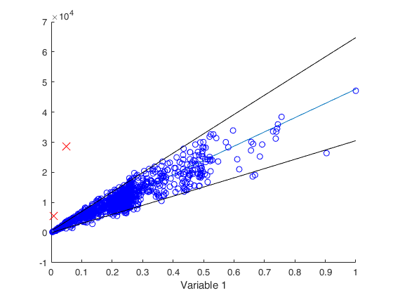
 Example of use of option bsb.
Example of use of option bsb.
close all
load tradeH.mat
y=tradeH{:,2};
X=tradeH{:,1};
X=X./max(X);
Z=log(X);
n=length(y);
bsb=1:n;
% outl = the outliers
outl=[225   660];
bsb(outl)=[];
% call of forecastH with option bsb
outFORE=forecastH(y,X,Z,'bsb',bsb);
Related Examples
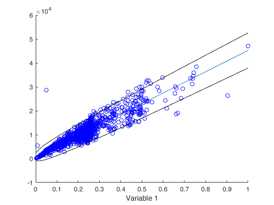
Example of use of option typeH.
Example of use of option typeH.
close all
load tradeH.mat
y=tradeH{:,2};
X=tradeH{:,1};
X=X./max(X);
Z=log(X);
% Use Harvery's parametrization
fore=forecastH(y,X,Z,'typeH','har');
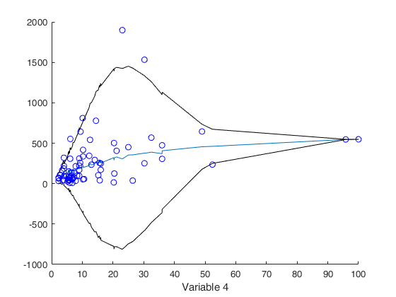
Monthly credit card expenditure for 100 individuals.
Monthly credit card expenditure for 100 individuals.Example of use of option selcolX
load('TableF91_Greene');
data=TableF91_Greene{:,:};
n=size(data,1);
% Linear regression of monthly expenditure on a constant, age, income
% its square and a dummy variable for home ownership using the 72
% observations for which expenditure was nonzero produces the residuals
% plotted below
X=zeros(n,4);
X(:,1)=data(:,3);%age
X(:,2)=data(:,6);% Own rent (dummy variable)
X(:,3)=data(:,4);% Income
X(:,4)=(data(:,4)).^2; %Income  square
y=data(:,5); % Monthly expenditure
% Select the 72 observations for which expenditure was nonzero
sel=y>0;
X=X(sel,:);
y=y(sel);
close all
disp('Multiplicative Heteroskedasticity Model')
% Plot of forecasts against column 4
warning('off')
out=forecastH(y,X,[3 4],'typeH','har','selcolX',4);
warning('on')
Multiplicative Heteroskedasticity Model
Input Arguments
Output Arguments
References
Greene, W.H. (1987), "Econometric Analysis", Prentice Hall. [5th edition, section 11.7.1 pp. 232-235, 7th edition, section 9.7.1 pp. 280-282]
Atkinson, A.C., Riani, M. and Torti, F. (2016), Robust methods for heteroskedastic regression, "Computational Statistics and Data Analysis", Vol. 104, pp. 209-222, http://dx.doi.org/10.1016/j.csda.2016.07.002 [ART]