regressHhar
regressHhar fits a multiple linear regression model with Harvey heteroskedasticity
Description
Examples
 regressHhar with all default options.
regressHhar with all default options.Monthly credit card expenditure for 100 individuals.
% Results in structure "OUT" coincides with "Maximum Likelihood
% Estimates" of table 11.3, page 235, 5th edition of Greene (1987).
% Results in structure "OLS" coincide with "Ordinary Least Squares
% Estimates" of table 11.3, page 235, 5th edition of Greene (1987).
load('TableF91_Greene');
data=TableF91_Greene{:,:};
n=size(data,1);
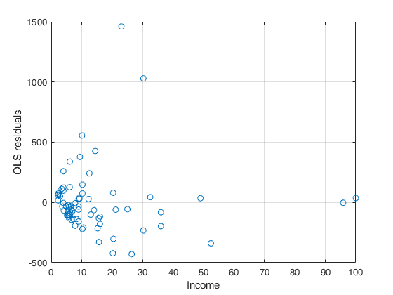
% Linear regression of monthly expenditure on a constant, age, income
% its square and a dummy variable for home ownership using the 72
% observations for which expenditure was nonzero produces the residuals
% plotted below.
X=zeros(n,4);
X(:,1)=data(:,3); % age
X(:,2)=data(:,6); % Own rent (dummy variable)
X(:,3)=data(:,4); % Income
X(:,4)=(data(:,4)).^2; % Income square
y=data(:,5); % Monthly expenditure
% Select the 72 observations for which expenditure was nonzero
sel=y>0;
X=X(sel,:);
y=y(sel);
whichstats={'r','tstat'};
OLS=regstats(y,X,'linear',whichstats);
r=OLS.r;
disp('Ordinary Least Squares Estimates')
LSest=[OLS.tstat.beta OLS.tstat.se OLS.tstat.t OLS.tstat.pval];
disp(LSest)
disp('Multiplicative Heteroskedasticity Model')
% The variables which enter the scedastic function are Income and
% Income square (that is columns 3 and 4 of matrix X).
out=regressHhar(y,X,[3 4]);
% Plot OLS residuals against Income (This is nothing but Figure 11.1 of
% Green (5th edition) p. 216).
plot(X(:,4),r,'o')
xlabel('Income')
ylabel('OLS residuals')
grid on
Ordinary Least Squares Estimates
 -237.1465  199.3517   -1.1896    0.2384
   -3.0818    5.5147   -0.5588    0.5781
   27.9409   82.9223    0.3370    0.7372
  234.3470   80.3660    2.9160    0.0048
  -14.9968    7.4693   -2.0078    0.0487

Multiplicative Heteroskedasticity Model
Related Examples
FGLS estimator.
FGLS estimator.Estimate a multiplicative heteroscedastic model using just one iteration that is find FGLS estimator (two step estimator).
% Data are monthly credit card expenditure for 100 individuals.
% Results in structure "out" coincide with estimates of row
% "$\sigma^2_i=\sigma^2 \exp(z' \alpha)$" in table 11.2, page 231, 5th edition of
% Greene (1987).
load('TableF91_Greene');
data=TableF91_Greene{:,:};
n=size(data,1);
% Linear regression of monthly expenditure on a constant, age, income and
% its square and a dummy variable for home ownership using the 72
% observations for which expenditure was nonzero produces the residuals
% plotted below.
X=zeros(n,4);
X(:,1)=data(:,3); % age
X(:,2)=data(:,6); % Own rent (dummy variable)
X(:,3)=data(:,4); % Income
X(:,4)=(data(:,4)).^2; % Income  square
y=data(:,5); % Monthly expenditure
% Select the 72 observations for which expenditure was nonzero
sel=y>0;
X=X(sel,:);
y=y(sel);
out=regressHhar(y,X,[3 4],'msgiter',1,'maxiter',1);
Regression parameters beta
Coeff.   SE     t-stat
 -117.8675   50.4970   -2.3341
   -1.2337    1.2707   -0.9709
   50.9498   26.3050    1.9369
  145.3045   23.0917    6.2925
   -7.9383    1.8611   -4.2653

Scedastic parameters gamma from first iteration
Coeff.
    4.1374
    2.4857
   -0.2449
Input Arguments
Output Arguments
More About
References
Greene W.H. (1987), Econometric Analysis, Prentice Hall. [5th edition, section 11.7.1 pp. 232-235, 7th edition, section 9.7.1 pp. 280-282].