Response variable, specified as
a vector of length n, where n is the number of
observations. Each entry in y is the response for the
corresponding row of X.
Missing values (NaN's) and infinite values (Inf's) are
allowed, since observations (rows) with missing or infinite
values will automatically be excluded from the
computations.
Data Types: single| double
Matrix of explanatory
variables (also called 'regressors') of dimension n x (p-1)
where p denotes the number of explanatory variables
including the intercept.
Rows of X represent observations, and columns represent
variables. By default, there is a constant term in the
model, unless you explicitly remove it using input option
intercept, so do not include a column of 1s in X. Missing
values (NaN's) and infinite values (Inf's) are allowed,
since observations (rows) with missing or infinite values
will automatically be excluded from the computations.
Data Types: single| double
Specify optional comma-separated pairs of Name,Value arguments.
Name is the argument name and Value
is the corresponding value. Name must appear
inside single quotes (' ').
You can specify several name and value pair arguments in any order as
Name1,Value1,...,NameN,ValueN.
Example:
 'bsbmfullrank',false
, 'bonflev',0.99
, 'h',round(n*0,75)
, 'init',100 starts monitoring from step m=100
, 'intercept',false
, 'lms',1
, 'msg',false
, 'nocheck',true
, 'nsamp',1000
, 'threshoutX',1
, 'weak',true
, 'plots',1
, 'bivarfit','2'
, 'labeladd','1'
, 'multivarfit','1'
, 'nameX',{'NameVar1','NameVar2'}
, 'namey','NameOfResponse'
, 'tag',{'plmdr' 'plyXplot'};
,
This option tells
how to behave in case subset at step m
(say bsbm) produces a singular X. In other words,
this options controls what to do when rank(X(bsbm,:)) is
smaller then number of explanatory variables. If
bsbmfullrank =true (default) these units (whose number is
say mnofullrank) are constrained to enter the search in
the final n-mnofullrank steps else the search continues
using as estimate of beta at step m the estimate of beta
found in the previous step.
Example: 'bsbmfullrank',false
Data Types: logical
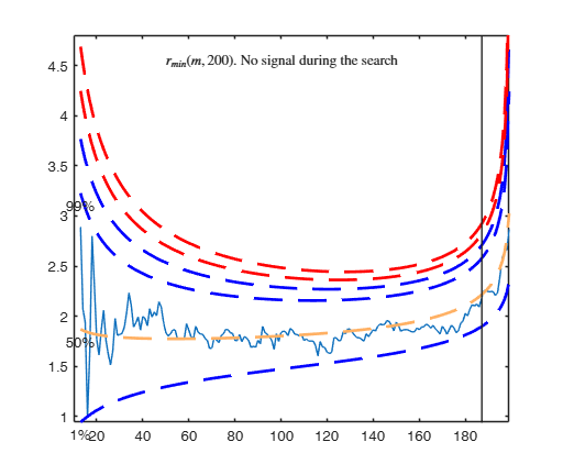
Option to be used if the distribution of the data is
strongly non normal and, thus, the general signal
detection rule based on consecutive exceedances cannot be
used. In this case bonflev can be:
- a scalar smaller than 1 which specifies the confidence
level for a signal and a stopping rule based on the
comparison of the minimum MD with a
Bonferroni bound. For example if bonflev=0.99 the
procedure stops when the trajectory exceeds for the
first time the 99% bonferroni bound.
- A scalar value greater than 1. In this case the
procedure stops when the residual trajectory exceeds
for the first time this value.
Default value is '', which means to rely on general rules
based on consecutive exceedances.
Example: 'bonflev',0.99
Data Types: double
h is an integer
greater or equal than p but smaller then n. Generally if
the purpose is outlier detection h=[0.5*(n+p+1)] (default
value). h can be smaller than this threshold if the
purpose is to find subgroups of homogeneous observations.
In this function the LTS/LMS estimator is used just to
initialize the search.
Example: 'h',round(n*0,75)
Data Types: double
It specifies the initial
subset size to start monitoring exceedances of minimum
deletion residual, if init is not specified it set equal
to:
p+1, if the sample size is smaller than 40;
min(3*p+1,floor(0.5*(n+p+1))), otherwise.
Example: 'init',100 starts monitoring from step m=100
Data Types: double
Indicator for the constant term (intercept) in the fit,
specified as the comma-separated pair consisting of
'Intercept' and either true to include or false to remove
the constant term from the model.
Example: 'intercept',false
Data Types: boolean
lms specifies the criterion to use to find the initial
subset to initialize the search (LMS, LTS with
concentration steps, LTS without concentration steps
or subset supplied directly by the user).
The default value is 1 (Least Median of Squares
is computed to initialize the search). On the other hand,
if the user wants to initialize the search with LTS with
all the default options for concentration steps then
lms=2. If the user wants to use LTS without
concentration steps, lms can be a scalar different from 1
or 2. If lms is a struct it is possible to control a
series of options for concentration steps (for more
details see option lms inside LXS.m)
LXS.
If, on the other hand, the user wants to initialize the
search with a prespecified set of units there are two
possibilities:
1) lms can be a vector with length greater than 1 which
contains the list of units forming the initial subset. For
example, if the user wants to initialize the search
with units 4, 6 and 10 then lms=[4 6 10];
2) lms is a struct that contains a field named bsb which
contains the list of units to initialize the search. For
example, in the case of simple regression through the
origin with just one explanatory variable, if the user
wants to initialize the search with unit 3 then
lms=struct;
Example: 'lms',1
Data Types: double
It controls whether
to display or not messages on the screen
If msg==true (default) messages are displayed on the screen about
step in which signal took place
else no message is displayed on the screen.
Example: 'msg',false
Data Types: logical
If nocheck is equal to
true no check is performed on matrix y and matrix X.
Notice that y and X are left unchanged. In other words
the additional column of ones for the intercept is not
added. As default nocheck=false.
Example: 'nocheck',true
Data Types: double
If nsamp=0 all subsets will be extracted.
They will be (n choose p).
If the number of all possible subset is <1000 the
default is to extract all subsets otherwise just 1000.
Example: 'nsamp',1000
Data Types: double
If the design matrix X contains several high leverage units
(that is units which are very far from the bulk of the
data), it may happen that the best subset of LXS may include some
of these units, or it may happen that these units have a
deletion residual which is very small due to their
extremely high value of . bonflevoutX=1 imposes the
constraints that:
1) the extracted subsets which contain
at least one unit declared as outlier in the X space by FSM
using a Bonferronized confidence level of 0.99
are removed from the list of candidate subsets to find the
LXS solution.
2) imposes the constraint that h_i(m^*)
cannot exceed 10 \times p/m.
If threshoutX is a structure, it contains the following
fields:
| Value |
Description |
bonflevoutX |
specifies the Bonferronized
confidence level to be used to find the outliers in the X
space. If this field is not present, a 99 percent
confidence level is used.
|
threshlevoutX |
specifies the threshold to bound
the effect of high leverage units in the computation of
deletion residuals. In the computation of
the quantity h_i(m^*) = x_i^T\{X(m^*)^TX(m^*)\}^{-1}x_i,
i \notin S^{(m)}_*, units which are very far from the bulk of
the data (represented by X(m^*)) will have a huge value
of h_i(m^*) and consequently, the deletion of residuals.
In order to tackle this problem it is possible to put a
bound to the value of h_i(m^*). For example
threshoutX.threshlevoutX=r imposes the constraint that h_i(m^*)
cannot exceed r \times p/m. If this field is not present
the default threshold of 10 is imposed.
|
Example: 'threshoutX',1
Data Types: double
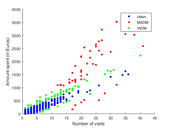
If weak=false default FSRcore values are used,
if weak=true 'stronger' quantiles are used as a
decision rule to trim outliers and VIOM outliers
are the ones entering the Search after the first signal.
Example: 'weak',true
Data Types: logical
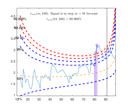
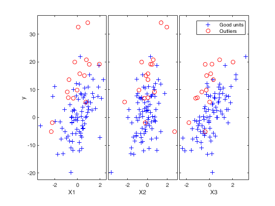
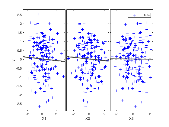
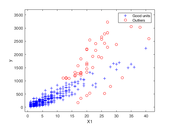
If plots=1 (default) the plot of minimum deletion
residual with envelopes based on n observations and the
yXplot matrix with the outliers highlighted is
produced.
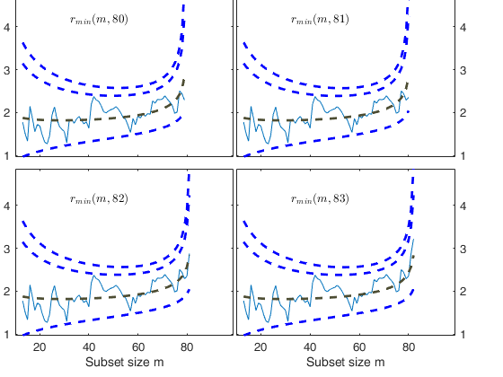
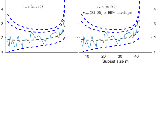
If plots=2 the user can also monitor the intermediate
plots based on envelope superimposition.
Else no plot is produced.
Example: 'plots',1
Data Types: double
This option adds
one or more least squares lines, based on
SIMPLE REGRESSION of y on Xi, to the plots of y|Xi.
bivarfit = ''
is the default: no line is fitted.
bivarfit = '1'
fits a single ols line to all points of each bivariate
plot in the scatter matrix y|X.
bivarfit = '2'
fits two ols lines: one to all points and another to
the group of the genuine observations. The group of the
potential outliers is not fitted.
bivarfit = '0'
fits one ols line to each group. This is useful for the
purpose of fitting mixtures of regression lines.
bivarfit = 'i1' or 'i2' or 'i3' etc. fits
an ols line to a specific group, the one with
index 'i' equal to 1, 2, 3 etc. Again, useful in case
of mixtures.
Example: 'bivarfit','2'
Data Types: char
If this option is
'1', we label the outliers with the
unit row index in matrices X and y. The default value is
labeladd='', i.e. no label is added.
Example: 'labeladd','1'
Data Types: char
This option adds one or more least square lines, based on
MULTIVARIATE REGRESSION of y on X, to the plots of y|Xi.
multivarfit = ''
is the default: no line is fitted.
multivarfit = '1'
fits a single ols line to all points of each bivariate
plot in the scatter matrix y|X. The line added to the
scatter plot y|Xi is avconst + Ci*Xi, where Ci is the
coefficient of Xi in the multivariate regression and
avconst is the effect of all the other explanatory
variables different from Xi evaluated at their centroid
(that is overline{y}'C))
multivarfit = '2'
equal to multivarfit ='1' but this time we also add the
line based on the group of unselected observations
(i.e. the normal units).
Example: 'multivarfit','1'
Data Types: char
Cell
array of strings of length p containing the labels of
the variables of the regression dataset. If it is empty
(default) the sequence X1, ..., Xp will be created
automatically
Example: 'nameX',{'NameVar1','NameVar2'}
Data Types: cell
String containing the
label of the response
Example: 'namey','NameOfResponse'
Data Types: char
This option enables to add a tag to the plots which are
created. The default tag names are:
fsr_mdrplot for the plot of mdr based on all the
observations;
fsr_yXplot for the plot of y against each column of X
with the outliers highlighted;
fsr_resuperplot for the plot of resuperimposed envelopes. The
first plot with 4 panel of resuperimposed envelopes has
tag fsr_resuperplot1, the second fsr_resuperplot2 ...
If tag is character or a cell of characters of length 1,
it is possible to specify the tag for the plot of mdr
based on all the observations;
If tag is a cell of length 2 it is possible to control
both the tag for the plot of mdr based on all the
observations and the tag for the yXplot with outliers
highlighted.
If tag is a cell of length 3 the third element specifies
the names of the plots of resuperimposed envelopes.
Example: 'tag',{'plmdr' 'plyXplot'};
Data Types: char or cell
Vector with two elements
minimum and maximum on the x axis. Default value is ''
(automatic scale)
Example: 'xlim',[0,10] sets the minimum value to 0 and the
max to 10 on the x axis
Data Types: double
Vector with two elements
controlling minimum and maximum on the y axis.
Default value is '' (automatic scale)
Example: 'ylim',[0,10] sets the minimum value to 0 and the
max to 10 on the y axis
Data Types: double
 FSR with optional arguments.