inversegamcdf
inversegamcdf computes inverse-gamma cumulative distribution function.
Description
Examples
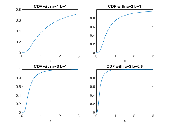
 Plot the cdf for 4 different combinations of parameter values.
Plot the cdf for 4 different combinations of parameter values.
x=(0:0.001:3)';
a=[1,2,3,3];
b=[1,1,1,0.5];
Y=zeros(length(x),length(a));
for i=1:length(x)
Y(i,:)=inversegamcdf(x(i),a,b);
end
for j=1:4
subplot(2,2,j)
plot(x,Y(:,j))
title(['CDF with a=' num2str(a(j)) ' b=' num2str(b(j))])
xlabel('x')
end
Compare the results using option nocheck=1.
Compare the results using option nocheck=1.
x=(0:0.001:3)';
a=[1,2,3,50,100,10000];
b=[1,10,100,0.05,10,800];
Y=zeros(length(x),length(a));
Ychk=Y;
for i=1:length(x)
Y(i,:)=inversegamcdf(x(i),a,b);
Ychk(i,:)=inversegamcdf(x(i),a,b,1);
end
disp('Maximum absolute difference is:');
disp(max(max(abs(Y-Ychk))));
Maximum absolute difference is:
          0.00