inversegamcdf
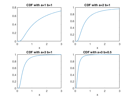
inversegamcdf computes inverse-gamma cumulative distribution function.
Description
Examples
 Compare the results using option nocheck=1.
 Compare the results using option nocheck=1.
x=(0:0.001:3)';
a=[1,2,3,50,100,10000];
b=[1,10,100,0.05,10,800];
Y=zeros(length(x),length(a));
Ychk=Y;
for i=1:length(x)
Y(i,:)=inversegamcdf(x(i),a,b);
Ychk(i,:)=inversegamcdf(x(i),a,b,1);
end
disp('Maximum absolute difference is:');
disp(max(max(abs(Y-Ychk))));
Maximum absolute difference is:
0.00
Input Arguments
x — Value at which the cdf must be evaluated.
Scalar, vector or matrix 3D array of the same size of x and b.
A scalar input functions as a constant matrix of the same size as the other input.
See the section called "More About:" for more details about the inverse gamma distribution.
Data Types: single | double
a — shape parameter of the inverse-gamma distribution.
Scalar, vector or matrix 3D array of the same size of x and b.
A scalar input functions as a constant matrix of the same size as the other input.
See the section called "More About:" for more details about the inverse gamma distribution.
Data Types: single | double
b — scale parameter b of the inverse-gamma distribution.
Scalar, vector or matrix 3D array of the same size of x and a.
A scalar input functions as a constant matrix of the same size as the other input.
Unlike the Gamma distribution, which contains a somewhat similar exponential term, $b$ is a scale parameter as the distribution function satisfies:
\[ f_{IG}(x,a,b)=\frac{f(x/b,a,1)}{b} \]See the section called "More About:" for more details about the inverse gamma distribution.
Data Types: single | double
Optional Arguments
nocheck — Check input arguments.
Scalar.
If nocheck is equal to 1 no check is performed and input and the cdf is evaluated directly through MATLAB buit in function gammainc else we use MATLAB function gamcdf
Example: 'nocheck',1
Data Types: double
Output Arguments
y —CDF value.
Scalar, vector or
Scalar, vector or $y=\int_0^x f_{IG}(t | a,b) dt$ is the value of the cdf of the inverse gamma distribution evaluated at x
More About
Additional Details
The cdf of the inverse gamma distribution defined over the support $x>0$ with shape parameter $a$ and scale parameter $b$ is \[ F_{IG}(x, a, b) =\int_0^x t^{-a -1} \exp (-b/t) \frac{b^a}{\Gamma(a)} dt \]
inversegamcdf computes the inverse-gamma cdf at each of the values in x using the corresponding shape parameters in a and scale parameters in b. x, a, and b can be vectors, matrices, or multidimensional arrays that all have the same size. A scalar input is expanded to a constant array with the same dimensions as the other inputs. The parameters in a and b must all be positive, and the values in x must lie on the interval $[0, \infty)$.
Note that $F_{IG}(x,a,b)=\frac{\Gamma(a,b/x)}{\Gamma(\alpha)}$ therefore Therefore, the CDF for an inverse Gamma distribution can be computed using the incomplete gamma function (also called regularized gamma function, i.e. MATLAB function gammainc) of course keeping into account that we need the upper tail.
The chief use of the inverse gamma distribution is in Bayesian statistics, where the distribution arises as the marginal posterior distribution for the unknown variance of a normal distribution if an uninformative prior is used; and as an analytically tractable conjugate prior if an informative prior is required.
Relation with the Gamma distribution.
If $X \sim Gamma(a,b)$ then $\frac{1}{X} \sim$ inverse-gamma distribution with paramters $a$ and $1/b$.
