mWNChygernd
mWNChygernd returns random arrays from the Wallenius non central hypergeometric distribution
Syntax
Description
This function calls function CMultiWalleniusNCHypergeometricrnd which is a translation into MATLAB of the corresponding C++ function of Fog (2008).
The notation which is used in mWNChygernd and the order of the arguments is the one of MATLAB hyge. The notation which is used inside CMultiWalleniusNCHypergeometricrnd is the original one of Fog.
To illustrate the meaning of Wallenius and Fisher' function parameters, let's use the classical biased urn example, with $K$ red balls and $M-K$ white balls, totalling $M$ balls. $n$ balls are drawn at random from the urn without replacement. Each red ball has the weight $\omega_{1}$, and each white ball has the weight $\omega_{2}$; the probability ratio of red over white balls is then given by $odds = \omega_{1} / \omega_{2}$. Note that the odds are fixed once and for all during the drawings.
If the balls are taken one by one, the probability (say $p_1$) that the first ball picked is red is equal to the weight fraction of red balls:
\[ p_1= \frac{K w_1}{K w_1 + (M-K) w_2} \]In the Wallenius distribution the probability that the second ball picked is red depends on whether the first ball was red or white. If the first ball was red then the above formula is used with $K$ reduced by one. If the first ball was not red then the above formula is used with $M-K$ reduced by one. The number of red balls that we get in this experiment is a random variable with Wallenius' noncentral hypergeometric distribution.
The important fact that distinguishes Wallenius' distribution is that there is competition between the balls. The probability that a particular ball is taken in a particular draw depends not only on its own weight, but also on the total weight of the competing balls that remain in the urn at that moment. And the weight of the competing balls depends on the outcomes of all preceding draws. In the Fisher model, the fates of the balls are independent and there is no dependence between draws. One may as well take all $n$ balls at the same time. Each ball has no "knowledge" of what happens to the other balls.
More formally, if the total number $n$ of balls taken is not known before the experiment (i.e n is determined just after the experiment), then the conditional distribution of the number of taken red balls for given $n$ is Fisher's noncentral hypergeometric distribution.
These two distributions have important applications in evolutionary biology and population genetics. If animals of a particular species are competing for a limited food resource so that individual animals are dying one by one until there is enough food for the remaining animals, and if there are different variants of animals with different chances of finding food, then we can expect the animals that die to follow a Wallenius noncentral hypergeometric distribution. Fisher’s noncentral hypergeometric distribution may be used instead of Wallenius distribution in cases where the fates of the individual animals are independent and the total number of survivors is known or controlled as part of a simulation experiment (Fog 2008).
Wallenius distribution is a general model of biased sampling. Fisher’s noncentral hypergeometric distribution is used for statistical tests on contingency tables where the marginals are fixed (McCullagh and Nelder, 1983).
The multivariate Fishers and Wallenius noncentral hypergeometric distribution, are referred to the case where the type of different balls is greater than 2 and each ball has a different probability.
The two distributions are both equal to the (multivariate) hypergeometric distribution when the odds ratio is 1.
Examples
 Problem description.
Problem description.We have 70 balls in a urn of 3 different colors.
% Initially in the urn we have 20 red balls, 30 white and 20 black balls.
m=[20,30,20];
% The weight of each color is 1, 2,5 and 1.8
w=[1, 2.5, 1.8];
% n=number of balls which are taken
n=10;
% Generate a random variate from this distribution
r = mWNChygernd(m,w, n);
disp(r);
1.00 6.00 3.00
Generate 5 random variates from a multivariate non central Wallenius distribution.
Generate 5 random variates from a multivariate non central Wallenius distribution.m = number of balls of each type in the urn.
m=[20,30,20, 10];
% w = vector containing the weight of each color
w=[1, 2.5, 1.8, 100];
% n=number of balls which are taken
n=10;
% Generate 5 random variates from this distribution
ntrials=5;
R = mWNChygernd(m,w, n, ntrials);
% R is matrix of size ntrials-by-length(m)
disp(R);
             0          1.00             0          9.00
             0          1.00          1.00          8.00
          1.00          1.00             0          8.00
             0          1.00          1.00          8.00
             0          2.00             0          8.00
Check agreement between theoretical and empirical relative frequencies.
Check agreement between theoretical and empirical relative frequencies.define the weights for each color
weights=[5,2,1]';
% Define urn composition
m=[12 25 18];
% Number of balls which are drawn.
numberBallsExtracted=5;
% number of random variates which are generated.
ntrials=100000;
% Define all possible cases in which numberBallsExtracted is equal 5
% Length of each permutation
numcolors = length(m);
% Create all possible permutations (with repetition) of numcolors
C = cell(numcolors, 1);         % Preallocate a cell array
x=0:numberBallsExtracted;
[C{:}] = ndgrid(x);     % Create grids of values
Y = cellfun(@(x){x(:)}, C); % Convert grids to column vectors
Y = [Y{:}];   % Create matrix with all possible permutations with repetion
% Extract from Y the rows whose sum is equal to numberBallsExtracted
boo=sum(Y,2)==numberBallsExtracted;
Ysel=Y(boo,:);
% Find the probability of each row of matrix Ysel
Wpdf=mWNChygepdf(Ysel,m,weights);
% Make sure that the sum of all probabilities is to (up to a certain
% tolerance)
tol=1e-08;
assert(abs(sum(Wpdf)-1)<tol,"FSDA:Sum of densities is not equal to 1")
Outcomes=cellstr((num2str(Ysel)));
% Generate a matrix of ntrials random variates
Wrnd=mWNChygernd(m,weights,numberBallsExtracted,ntrials);
% Compute the frequency distribution (pivot table) of observed outcomes
Rd=cellstr(num2str(Wrnd));
Rdtable=table(Rd);
OutcomesObs=pivot(Rdtable,'Rows','Rd');
% Make sure that there is a matching between the rows of theoretical and
% empirical frequencies
OutcomesO=cell2mat(strrep((OutcomesObs{:,1}),' ',''))-48;
[int,ia,ib]=intersect(Outcomes,OutcomesObs{:,1});
% Define the table which will contain both theoretical (density values) and
% empirical frequencies
Freq=table('Size',[size(Ysel,1),2],'VariableTypes',{'double' 'double'});
Freq.Properties.RowNames=Outcomes;
Freq{:,1}=Wpdf;
Freq{ia,2}=OutcomesObs{:,2}/ntrials;
Freq.Properties.VariableNames=["Densities" "Relative frequencies"];
% Create categorical object in order to label x axis
OutcomesC=categorical(Outcomes,Outcomes);
bar(OutcomesC,Freq{:,1:2})
legend(["Theoretical probabilities" "Relative frequencies"])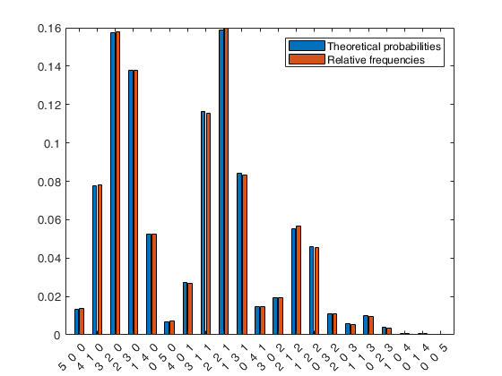
Input Arguments
Output Arguments
References
Fog, A. (2008), Calculation Methods for Wallenius' Noncentral Hypergeometric Distribution, "Communications in Statistics - Simulation and Computation", Vol. 37, pp. 258-273.
See Also
WNChygepdf
|
WNChygecdf
|
WNChygeinv
|
WNChygernd
|
FNChygepdf
|
FNChygecdf
|
FNChygeinv
|
FNChygernd