mcdCorAna
mcdCorAna computes Minimum Covariance Determinant in correspondence analysis
Syntax
Description
Examples
 mcdCorAna with bdp=0.
mcdCorAna with bdp=0.
N=[  69    46    41    13    22    18
29    52    45     3     5     3
19    55    47     2     3     1
50    22    19     8    10     7
25    38    33     2     4     3
30     2     1    45     8     2
35     6     5    32     5     2
28    12     7     7     5     4
26    12    11    11     4     3
21     6     4     3     3     2];
rowlab={'Teens' 'PicksYouUp' 'Energy' 'EnjoyLife' ...
'WhenTired' 'Kids' 'Fun' 'Refreshes' ...
'CheersYouUp' 'Relax'};
collab={'Coke' 'V' 'RedBull' 'Fanta' 'Pepsi' 'DietCoke'};
Ntable=array2table(N,'RowNames',rowlab,'VariableNames',collab);
RAW=mcdCorAna(Ntable,'bdp',0);
% Note that in this case RAW.md is equal to
% out.OverviewRows.Inertia./out.OverviewRows.Mass
% out = output from traditional correspondence analysis.
out=CorAna(Ntable,'dispresults',false,'plots',0);
d2=out.OverviewRows.Inertia./out.OverviewRows.Mass;
disp('Square distance of each row profile from the centroid')
disp([RAW.md d2])
The MCD estimates are equal to the classical estimates h=n=1036
Square distance of each row profile from the centroid
0.10 0.10
0.29 0.29
0.52 0.52
0.09 0.09
0.24 0.24
1.65 1.65
0.80 0.80
0.12 0.12
0.05 0.05
0.25 0.25
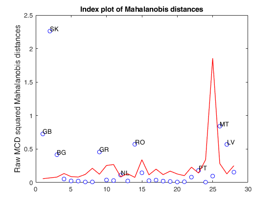
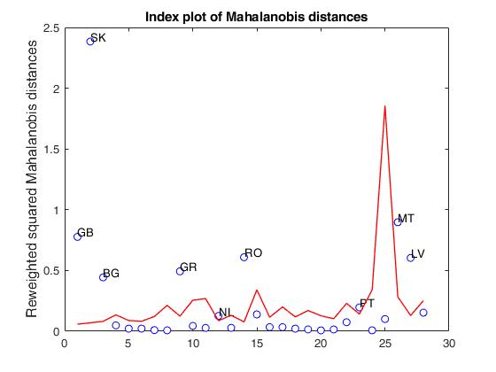
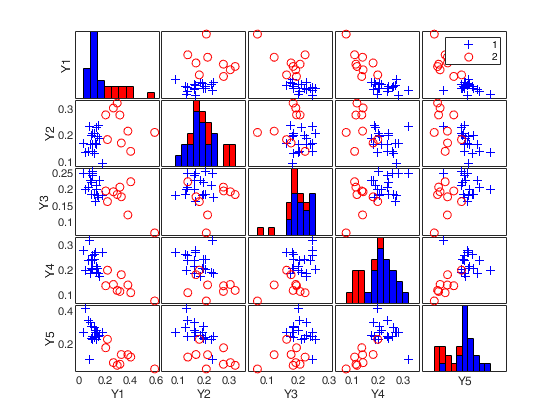
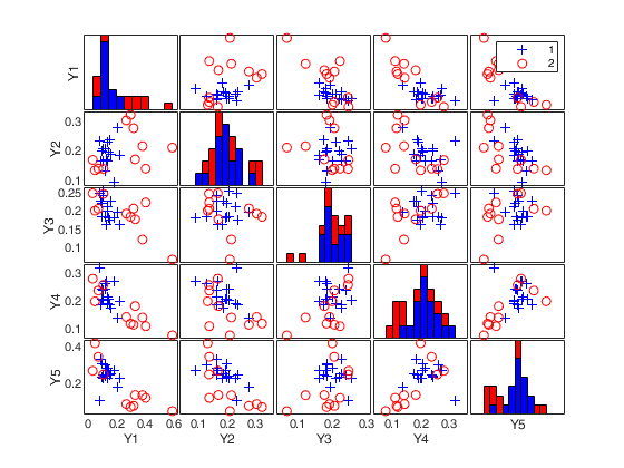
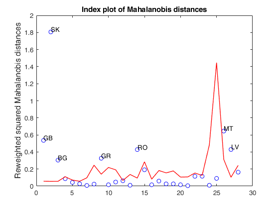
Raw and reweighted MCD.
Raw and reweighted MCD.
load clothes.mat
[RAW,REW]=mcdCorAna(clothes,'plots',1);
Total estimated time to complete MCD: 0.26 seconds

Related Examples
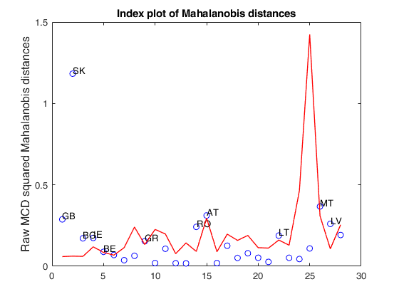
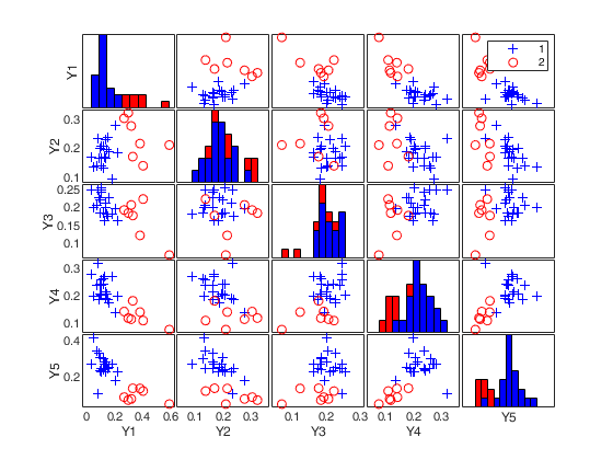
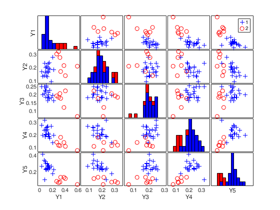
Example 2 of findEmpiricalEnvelope a struct
load clothes.
Example 2 of findEmpiricalEnvelope a struct
load clothes.load clothes.mat findEmp=struct; % Generate 500 contingency tables findEmp.nsimul=500; % Under the null hypothesis of independence findEmp.underH0=true; % Store the nsimul robust distances sorted (for each row) findEmp.StoreSim=true; % Detect outlying rows using a confidence level of 0.999 conflev=0.999; [RAW,REW]=mcdCorAna(clothes,'plots',1,'findEmpiricalEnvelope',findEmp,'conflev',conflev,'bdp',0.1);
Total estimated time to complete MCD:  0.02 seconds
Finding empirical bands
Input Arguments
Output Arguments
More About
References
Greenacre, M.J. (1993), "Correspondence Analysis in Practice", London, Academic Press.
Riani, M, Atkinson A.C., Torti, F., Corbellini A. (2023), Robust Correspondence Analysis, "Journal of the Royal Statistical Society Series C: Applied Statistics", Vol. 71, pp. 1381–1401, https://doi.org/10.1111/rssc.12580