mcdeda
mcdeda monitors Minimum Covariance Determinant for a series of values of bdp
Syntax
Description
Monitoring reweighted MD using two different confidence levels for reweighting.RAW
=mcdeda(Y,
Name, Value)
Examples
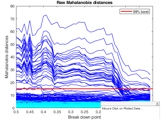
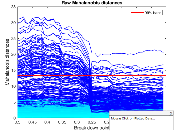
 Example of monitoring of raw and reweighted Mahalanobis distances.
Example of monitoring of raw and reweighted Mahalanobis distances.This example enables to obtain Figure 6 of CRAC2018.
Y = load('geyser.txt');
% Reweighted MD found using a confidence band for raw Mahalanobis distances
% equal to 0.99
conflev=0.99;
[RAW,REW]=mcdeda(Y,'conflev',conflev,'msg',false);
fground=struct;
fground.funit='';
fground.fthresh=1000;
% Add a horizontal line corresponding to 99 per cent confidence band
conflevplot=0.99;
% Monitoring of raw (squared) Mahalanobis distances
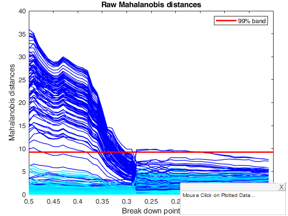
malfwdplot(RAW,'conflev',conflevplot,'fground',fground,'tag','rawMD')
title('Raw Mahalanobis distances')
% Monitoring of reweighted (squared) Mahalanobis distances
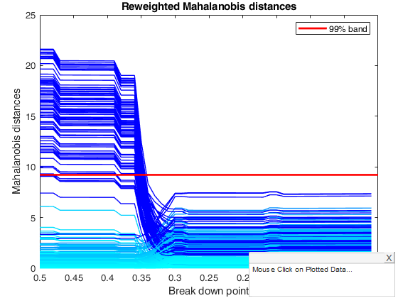
malfwdplot(REW,'conflev',conflevplot,'fground',fground,'tag','rewMD')
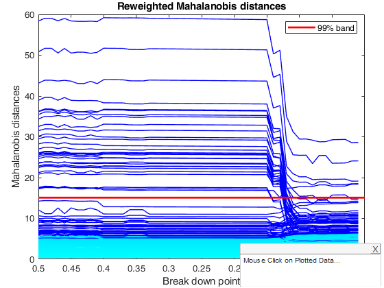
title('Reweighted Mahalanobis distances')
% Comment to the two plots. The squared robust raw distances initially decrease
% steadily. Then, at a bdp around 0.29 there is an abrupt change to a fit
% displaying two or three large distances which remains sensibly constant
% until the MLE is reached at bdp = 0.
% The plot for reweighted square Mahalanobis distances is much more stable
% than that for the crude MCD until 0.37, at which bdp there is a collapse
% to the MLE. The right-hand parts of both panels are similar. However, the
% distances for the crude MCD decreasing as successive observations are
% added to the subset used in fitting. On the other hand, the reweighted
% MCD shows three regions during which the distances are constant. In these
% regions the effect of changing the bdp in the (raw) first stage does not
% cause any change in the units chosen by the reweighting procedure
Monitoring reweighted MD using two different confidence levels for reweighting.
Monitoring reweighted MD using two different confidence levels for reweighting.This example enables to obtain Figure 7 of CRAC2018.
Y = load('geyser.txt');
% Reweighted MD found using a confidence band for raw Mahalanobis distances
% equal to 0.99
conflev=0.95;
[~,outrew095]=mcdeda(Y,'conflev',conflev,'msg',false);
fground=struct;
fground.funit='';
fground.fthresh=1000;
% Add a horizontal line corresponding to 99 per cent confidence band
conflevplot=0.99;
% Monitoring of raw (squared) Mahalanobis distances
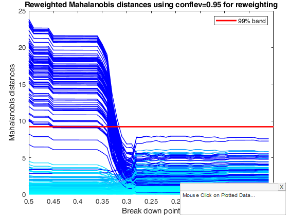
malfwdplot(outrew095,'conflev',conflevplot,'fground',fground,'tag','rewMDclev095')
title('Reweighted Mahalanobis distances using conflev=0.95 for reweighting')
conflev=0.999;
[~,outrew0999]=mcdeda(Y,'conflev',conflev,'msg',false);
% Monitoring of reweighted (squared) Mahalanobis distances
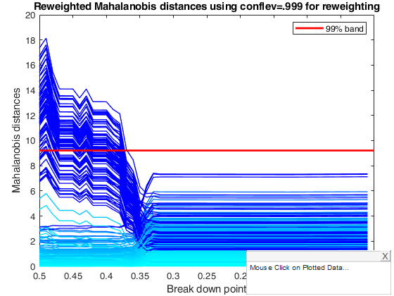
malfwdplot(outrew0999,'conflev',conflevplot,'fground',fground,'tag','rewMDclev0999')
title('Reweighted Mahalanobis distances using conflev=.999 for reweighting')
% The monitoring approach also helps to appreciate the effect of the
% threshold used in the reweighting step. Although the message conveyed by
% the two plots is broadly the same, the less efficient 95 per cent
% threshold produces a few more outliers and a neater separation between
% the two populations, while increasing efficiency in the reweighting step
% causes the inclusion of some contaminated units at a slightly larger bdp
% than 0.37

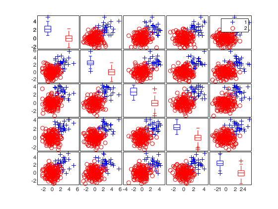
Example with mild contamination.
Example with mild contamination.This example enables to obtain left panel of Figure 15 of CRAC2018.
% In this simulated example there are 200 five-dimensional
% observations, all simulated with standard normal co-ordinates. Thirty of
% the observations had a displacement of 2.4 added to each co-ordinate. As
% a result the outliers are grouped, with virtually no overlap with the
% central 170 observations.
rng('default')
rng(100)
n=200;
v=5;
Xsel=randn(n,v);
kk=2.4;
numcont=30;
Xsel(1:numcont,:)=Xsel(1:numcont,:)+kk;
group=ones(n,1);
group(numcont+1:n)=2;
spmplot(Xsel,group,[],'box');
Y=Xsel;
conflev=0.99;
[outraw,outrew]=mcdeda(Y,'conflev',conflev,'msg',false);
fground=struct;
fground.funit='';
fground.fthresh=1000;
% Add a horizontal line corresponding to 99 per cent confidence band
conflevplot=0.99;
% Monitoring of raw (squared) Mahalanobis distances
malfwdplot(outraw,'conflev',conflevplot,'fground',fground,'tag','rawMD')
title('Raw Mahalanobis distances')
% Monitoring of reweighted (squared) Mahalanobis distances
malfwdplot(outrew,'conflev',conflevplot,'fground',fground,'tag','rewMD')
title('Reweighted Mahalanobis distances')
% The plot for the MCD is very jagged but does show the change in the
% pattern of distances around a bdp of 0.14. The monitoring plot for the
% reweighted MCD with a pointwise threshold of 0.99 is much the same as
% that for the original MCD, including a dramatic change at a bdp of 0.14
% The conclusion of this example is that most of the methods work well with
% a light amount of contamination well separated from the main body of the
% data. In general monitoring allows us to choose values of efficiency or
% breakdown point that give estimators that are as efficient as possible:
% that is, they exclude the outliers while fitting the “good”
% observations.
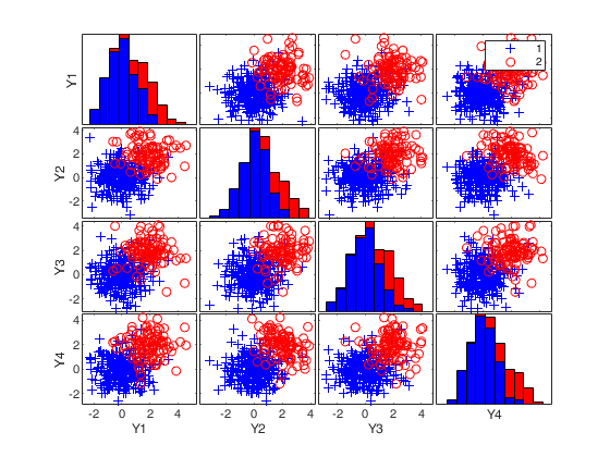
Example with strong contamination.
Example with strong contamination.This example enables to obtain Figure 20 of CRAC2018.
% In this example there are 400 four-dimensional standard normal random
% variables, one hundred of them being displaced by an amount 2 in each
% dimension. There is thus some overlap between the 25 per cent of outliers
% and the uncontaminated data.
rng('default')
rng(100)
n=400;
v=4;
Xsel=randn(n,v);
kk=2;
Xsel(301:400,:)=Xsel(301:400,:)+kk;
group=ones(n,1);
group(301:400)=2;
spmplot(Xsel,group);
Y=Xsel;
conflev=0.99;
[outraw,outrew]=mcdeda(Y,'conflev',conflev,'msg',false);
fground=struct;
fground.funit='';
fground.fthresh=1000;
% Add a horizontal line corresponding to 99 per cent confidence band
conflevplot=0.99;
% Monitoring of raw (squared) Mahalanobis distances
malfwdplot(outraw,'conflev',conflevplot,'fground',fground,'tag','rawMD')
title('Raw Mahalanobis distances')
% Monitoring of reweighted (squared) Mahalanobis distances
malfwdplot(outrew,'conflev',conflevplot,'fground',fground,'tag','rewMD')
title('Reweighted Mahalanobis distances')
% Comment to the plots: when bdp is 50%, 64 outliers are found using
% $\Chi^2_{4,0.99}$ (60 belong to the group of contaminated units). These
% are shown in the plot of raw Mahalanobis distances. Reweighting the
% output of this analysis leads to the detection of only 9 outliers (7
% belong to the group of contaminated units) as is shown in the plot of the
% reweighted distances. This plot shows how the distribution of distances
% for the 100 contaminated units is changed by the parameter estimates from
% reweighting. However, the distribution of these distances is even so
% quite distinct from those from the uncontaminated units. This effect of
% reweighting, which is not substantially affected by the choice of the
% reweighting threshold, is quite different from that shown in the case of
% lightly contaminated data, where weighted and unweighted analyses were
% comparable. However, monitoring the MCD is still very informative. The
% plot of raw distances shows a striking change around a bdp of 0.27 as the
% outliers start to be included in the central part of the data. In the
% monitoring plot for the reweighted MCD there is a change around a bdp of
% 0.28 when some Mahalanobis distances slightly increase in magnitude. For
% lower values of the bdp the plots in the two panels are similar; just 9
% observations are identified as outlying.
Input Arguments
Output Arguments
More About
References
Rousseeuw, P.J. (1984), Least Median of Squares Regression, "Journal of the American Statistical Association", Vol. 79, pp. 871-881.
Rousseeuw, P.J. and Van Driessen, K. (1999). A fast algorithm for the minimum covariance determinant estimator. Technometrics, 41:212-223.
Maronna, R.A., Martin D. and Yohai V.J. (2006), "Robust Statistics, Theory and Methods", Wiley, New York.
Cerioli A., Riani M., Atkinson A.C., Corbellini A. (2018). "The power of monitoring: how to make the most of a contaminated multivariate sample, "Statistical Methods and Applications (with discussion)", Vol. 27, pp. 559–587. [CRAC2018]