pcaFS
pcaFS performs Principal Component Analysis (PCA) on raw data.
Description
The main differences with respect to MATLAB function pca are:
1) accepts an input X also as table;
2) produces in table format the percentage of the variance explained single and cumulative of the various components and the associated Pareto plot, in order to decide about the number of components to retain.
3) returns the loadings in table format and shows them graphically.
4) provides guidelines about the automatic choice of the number of components;
5) returns the communalities for each variable with respect to the first k principal components in table format;
6) returns the orthogonal distance ($OD_i$) of each observation to the PCA subspace. For example, if the subspace is defined by the first two principal components, $OD_i$ is computed as:
\[ OD_i=|| z_i- V_{(2)} V_{(2)}' z_i || \]
where $z_i$ is the i-th row of the original centered (standardized) data matrix $Z$ of dimension $n \times p$ and $V_{(2)}=(v_1 v_2)$ is the matrix of size $p \times 2$ containing the first two eigenvectors of $Z'Z/(n-1)$. The observations with large $OD_i$ are not well represented in the space of the principal components.
7) returns the score distance $SD_i$ of each observation. For example, if the subspace is defined by the first two principal components, $SD_i$ is computed as:
\[ SD_i=\sqrt{(z_i'v_1)^2/l_1+ (z_i'v_2)^2/l_2 } \]
where $l_1$ and $l_2$ are the first two eigenvalues of $Z'Z/(n-1)$.
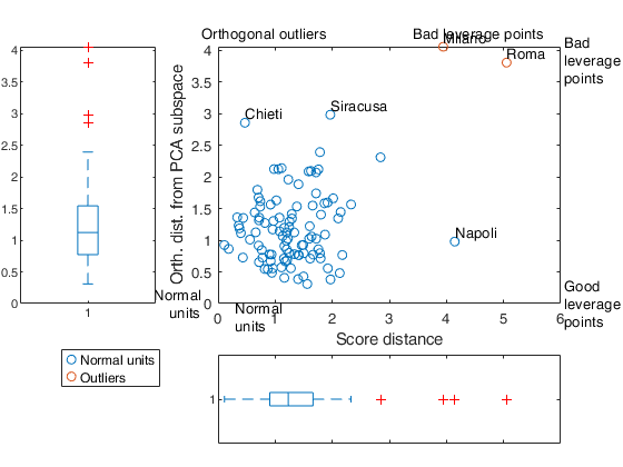
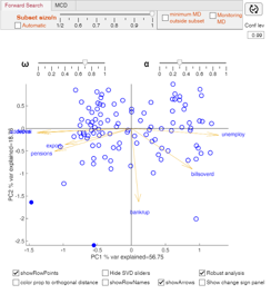
8) calls app biplotFS which enables to obtain an interactive biplot in which points, row labels or arrows can be shown or hidden. This app also gives the possibility of controlling the length of the arrows and the position of the row points through two interactive slider bars. In the app it is also possible to color row points depending on the orthogonal distance ($OD_i$) of each observation to the PCA subspace. If optional input argument bsb or bdp is specified, it is possible to have in the app two tabs which enable the user to select the breakdown point of the analysis or the subset size to use in the svd. The units which are declared as outliers or the units outside the subset are shown in the biplot with filled circles.
9) enables to deal with geographical information (latitude and longitude) or Shape polygons of the units.
Use of pcaFS on the ingredients dataset.out
=pcaFS(Y,
Name, Value)
Examples
 Use of pcaFS on the ingredients dataset.
Use of pcaFS on the ingredients dataset.
load hald
% Operate on the covariance matrix.
out=pcaFS(ingredients,'standardize',false,'biplot',0);
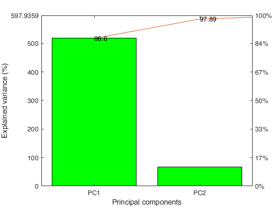
The first PC already explains more than 0.95^v variability
In what follows we still extract the first 2 PCs
Initial covariance matrix
Y1 Y2 Y3 Y4
_____ _____ _____ _____
Y1 1.00 0.23 -0.82 -0.25
Y2 0.23 1.00 -0.14 -0.97
Y3 -0.82 -0.14 1.00 0.03
Y4 -0.25 -0.97 0.03 1.00
Explained variance by PCs
Eigenvalues Explained_Variance Explained_Variance_cum
___________ __________________ ______________________
PC1 517.80 86.60 86.60
PC2 67.50 11.29 97.89
PC3 12.41 2.07 99.96
PC4 0.24 0.04 100.00
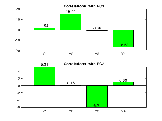
Loadings = correlations between variables and PCs
PC1 PC2
______ _____
Y1 1.54 5.31
Y2 15.44 0.16
Y3 -0.66 -6.21
Y4 -16.63 0.89
Communalities
PC1 PC2 PC1-PC2
______ _____ _______
Y1 2.38 28.17 30.55
Y2 238.39 0.03 238.41
Y3 0.44 38.51 38.94
Y4 276.60 0.79 277.39
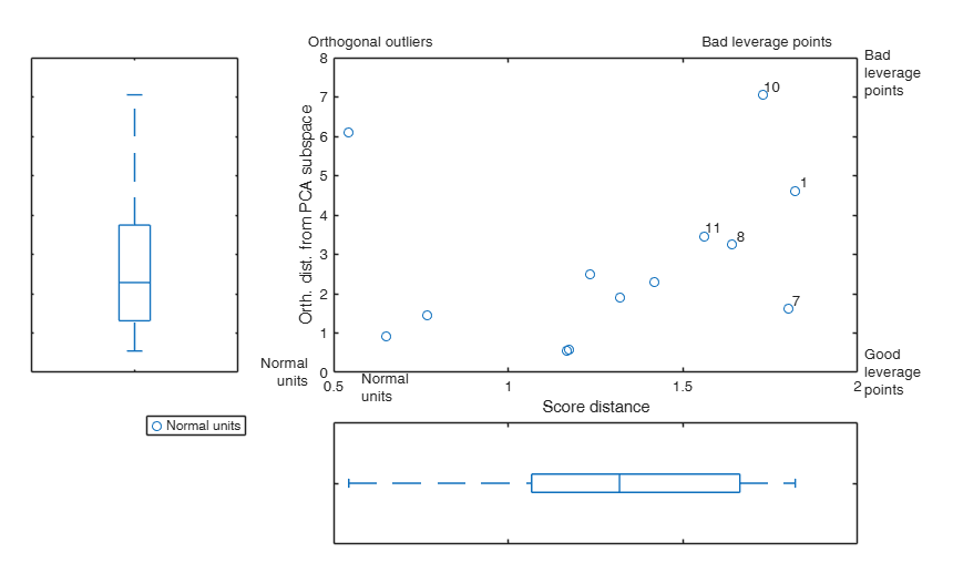
Units with the 5 largest values of (combined) score and orthogonal distance
10 1 7 8 11
Related Examples
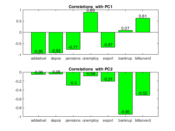
Use of pcaFS with option robust true.
Use of pcaFS with option robust true.
load citiesItaly;
% Use all default options
out=pcaFS(citiesItaly,'robust',true);
Initial correlation matrix
addedval depos pensions unemploy export bankrup billsoverd
________ _____ ________ ________ ______ _______ __________
addedval 1.00 0.91 0.73 -0.82 0.59 -0.04 -0.49
depos 0.91 1.00 0.70 -0.79 0.53 -0.03 -0.49
pensions 0.73 0.70 1.00 -0.52 0.35 0.24 -0.46
unemploy -0.82 -0.79 -0.52 1.00 -0.61 0.18 0.43
export 0.59 0.53 0.35 -0.61 1.00 0.07 -0.21
bankrup -0.04 -0.03 0.24 0.18 0.07 1.00 0.38
billsoverd -0.49 -0.49 -0.46 0.43 -0.21 0.38 1.00
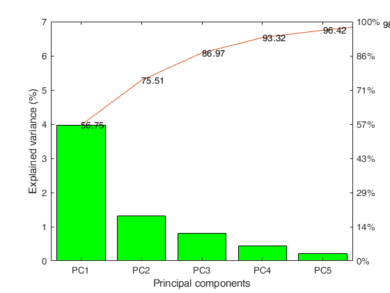
Explained variance by PCs
Eigenvalues Explained_Variance Explained_Variance_cum
___________ __________________ ______________________
PC1 3.97 56.75 56.75
PC2 1.31 18.76 75.51
PC3 0.80 11.45 86.97
PC4 0.45 6.36 93.32
PC5 0.22 3.10 96.42
PC6 0.17 2.43 98.85
PC7 0.08 1.15 100.00
Loadings = correlations between variables and PCs
PC1 PC2
_____ _____
addedval -0.95 -0.06
depos -0.93 -0.05
pensions -0.77 -0.30
unemploy 0.88 -0.09
export -0.67 -0.21
bankrup 0.07 -0.95
billsoverd 0.61 -0.52
Communalities
PC1 PC2 PC1-PC2
____ ____ _______
addedval 0.91 0.00 0.91
depos 0.86 0.00 0.87
pensions 0.60 0.09 0.69
unemploy 0.77 0.01 0.78
export 0.45 0.04 0.49
bankrup 0.01 0.89 0.90
billsoverd 0.38 0.27 0.65
Units with the 5 largest values of (combined) score and orthogonal distance
65 17 70 99 76
Use of pcaFS with options Latitude and Longitude.
Use of pcaFS with options Latitude and Longitude.
load citiesItaly2024.mat
X=citiesItaly2024;
% Retrieve Latitude and Longitude of each province
LatLong=X.Properties.UserData{2};
Latitude=LatLong(:,1);
Longitude=LatLong(:,2);
out=pcaFS(X,'Latitude',Latitude,'Longitude',Longitude);
The first PC already explains more than 0.95^v variability
In what follows we still extract the first 2 PCs
Initial correlation matrix
Deposit Bankrup UrbanFra Paym30D ElecPar QualLif Protest SalaryA SpendingA Employm AddedVa LowISEE
_______ _______ ________ _______ _______ _______ _______ _______ _________ _______ _______ _______
Deposit 1.00 -0.33 -0.70 0.72 0.58 0.76 -0.14 0.74 0.75 0.79 0.79 -0.76
Bankrup -0.33 1.00 0.26 -0.39 -0.13 -0.44 0.33 -0.18 -0.22 -0.32 -0.24 0.40
UrbanFra -0.70 0.26 1.00 -0.77 -0.74 -0.74 0.23 -0.74 -0.81 -0.90 -0.70 0.83
Paym30D 0.72 -0.39 -0.77 1.00 0.69 0.81 -0.35 0.74 0.79 0.80 0.63 -0.82
ElecPar 0.58 -0.13 -0.74 0.69 1.00 0.58 -0.16 0.64 0.78 0.73 0.55 -0.62
QualLif 0.76 -0.44 -0.74 0.81 0.58 1.00 -0.37 0.70 0.77 0.83 0.72 -0.86
Protest -0.14 0.33 0.23 -0.35 -0.16 -0.37 1.00 -0.14 -0.31 -0.31 -0.11 0.39
SalaryA 0.74 -0.18 -0.74 0.74 0.64 0.70 -0.14 1.00 0.85 0.80 0.86 -0.66
SpendingA 0.75 -0.22 -0.81 0.79 0.78 0.77 -0.31 0.85 1.00 0.92 0.78 -0.79
Employm 0.79 -0.32 -0.90 0.80 0.73 0.83 -0.31 0.80 0.92 1.00 0.81 -0.86
AddedVa 0.79 -0.24 -0.70 0.63 0.55 0.72 -0.11 0.86 0.78 0.81 1.00 -0.68
LowISEE -0.76 0.40 0.83 -0.82 -0.62 -0.86 0.39 -0.66 -0.79 -0.86 -0.68 1.00
Explained variance by PCs
Eigenvalues Explained_Variance Explained_Variance_cum
___________ __________________ ______________________
PC 1 8.02 66.82 66.82
PC 2 1.29 10.77 77.60
PC 3 0.77 6.45 84.05
PC 4 0.52 4.37 88.42
PC 5 0.36 3.00 91.42
PC 6 0.27 2.24 93.66
PC 7 0.24 1.98 95.64
PC 8 0.17 1.44 97.08
PC 9 0.13 1.04 98.12
PC10 0.10 0.82 98.94
PC11 0.09 0.73 99.66
PC12 0.04 0.34 100.00
Loadings = correlations between variables and PCs
PC1 PC2
_____ _____
Deposit -0.86 -0.10
Bankrup 0.38 -0.69
UrbanFra 0.89 0.10
Paym30D -0.89 0.11
ElecPar -0.77 -0.22
QualLif -0.89 0.18
Protest 0.34 -0.73
SalaryA -0.86 -0.27
SpendingA -0.93 -0.12
Employm -0.96 -0.04
AddedVa -0.84 -0.24
LowISEE 0.90 -0.17
Communalities
PC1 PC2 PC1-PC2
____ ____ _______
Deposit 0.73 0.01 0.74
Bankrup 0.15 0.47 0.62
UrbanFra 0.80 0.01 0.81
Paym30D 0.79 0.01 0.80
ElecPar 0.59 0.05 0.64
QualLif 0.80 0.03 0.83
Protest 0.11 0.53 0.65
SalaryA 0.74 0.07 0.82
SpendingA 0.86 0.01 0.88
Employm 0.91 0.00 0.92
AddedVa 0.71 0.06 0.76
LowISEE 0.82 0.03 0.85
Units with the 5 largest values of (combined) score and orthogonal distance
15 21 89 58 60


Use of pcaFS with option ShapeFile.
Use of pcaFS with option ShapeFile.Note that this option requires the Mapping Toolbox to be installed.
a=struct2table(ver);
MappingInstalled=any(string(a{:,1})=="Mapping Toolbox");
if MappingInstalled ==true
load citiesItaly2024.mat
X=citiesItaly2024;
ShapeFile=X.Properties.UserData{1};
out=pcaFS(X,"ShapeFile",ShapeFile,'biplot',0);
else
disp('This option requires that the "mapping toolbox" is installed')
end
The first PC already explains more than 0.95^v variability
In what follows we still extract the first 2 PCs
Initial correlation matrix
Deposit Bankrup UrbanFra Paym30D ElecPar QualLif Protest SalaryA SpendingA Employm AddedVa LowISEE
_______ _______ ________ _______ _______ _______ _______ _______ _________ _______ _______ _______
Deposit 1.00 -0.33 -0.70 0.72 0.58 0.76 -0.14 0.74 0.75 0.79 0.79 -0.76
Bankrup -0.33 1.00 0.26 -0.39 -0.13 -0.44 0.33 -0.18 -0.22 -0.32 -0.24 0.40
UrbanFra -0.70 0.26 1.00 -0.77 -0.74 -0.74 0.23 -0.74 -0.81 -0.90 -0.70 0.83
Paym30D 0.72 -0.39 -0.77 1.00 0.69 0.81 -0.35 0.74 0.79 0.80 0.63 -0.82
ElecPar 0.58 -0.13 -0.74 0.69 1.00 0.58 -0.16 0.64 0.78 0.73 0.55 -0.62
QualLif 0.76 -0.44 -0.74 0.81 0.58 1.00 -0.37 0.70 0.77 0.83 0.72 -0.86
Protest -0.14 0.33 0.23 -0.35 -0.16 -0.37 1.00 -0.14 -0.31 -0.31 -0.11 0.39
SalaryA 0.74 -0.18 -0.74 0.74 0.64 0.70 -0.14 1.00 0.85 0.80 0.86 -0.66
SpendingA 0.75 -0.22 -0.81 0.79 0.78 0.77 -0.31 0.85 1.00 0.92 0.78 -0.79
Employm 0.79 -0.32 -0.90 0.80 0.73 0.83 -0.31 0.80 0.92 1.00 0.81 -0.86
AddedVa 0.79 -0.24 -0.70 0.63 0.55 0.72 -0.11 0.86 0.78 0.81 1.00 -0.68
LowISEE -0.76 0.40 0.83 -0.82 -0.62 -0.86 0.39 -0.66 -0.79 -0.86 -0.68 1.00
Explained variance by PCs
Eigenvalues Explained_Variance Explained_Variance_cum
___________ __________________ ______________________
PC 1 8.02 66.82 66.82
PC 2 1.29 10.77 77.60
PC 3 0.77 6.45 84.05
PC 4 0.52 4.37 88.42
PC 5 0.36 3.00 91.42
PC 6 0.27 2.24 93.66
PC 7 0.24 1.98 95.64
PC 8 0.17 1.44 97.08
PC 9 0.13 1.04 98.12
PC10 0.10 0.82 98.94
PC11 0.09 0.73 99.66
PC12 0.04 0.34 100.00
Loadings = correlations between variables and PCs
PC1 PC2
_____ _____
Deposit -0.86 -0.10
Bankrup 0.38 -0.69
UrbanFra 0.89 0.10
Paym30D -0.89 0.11
ElecPar -0.77 -0.22
QualLif -0.89 0.18
Protest 0.34 -0.73
SalaryA -0.86 -0.27
SpendingA -0.93 -0.12
Employm -0.96 -0.04
AddedVa -0.84 -0.24
LowISEE 0.90 -0.17
Communalities
PC1 PC2 PC1-PC2
____ ____ _______
Deposit 0.73 0.01 0.74
Bankrup 0.15 0.47 0.62
UrbanFra 0.80 0.01 0.81
Paym30D 0.79 0.01 0.80
ElecPar 0.59 0.05 0.64
QualLif 0.80 0.03 0.83
Protest 0.11 0.53 0.65
SalaryA 0.74 0.07 0.82
SpendingA 0.86 0.01 0.88
Employm 0.91 0.00 0.92
AddedVa 0.71 0.06 0.76
LowISEE 0.82 0.03 0.85
Units with the 5 largest values of (combined) score and orthogonal distance
15 21 89 58 60


