simulateLM
simulateLM simulates linear regression data with pre-specified values of statistical indexes.
Description
simulateLM simulates linear regression data. It is possible to specify: 1) the requested value of R2 (or equivalently its SNR);
2) the values of the beta coefficients (possibly sparse);
3) the correlation (covariance) matrix among the explanatory variables.
4) the value of the intercept term.
5) the distribution to use to generate the Xs;
6) the distribution to use to generate the ys.
7) the MSOM contamination in Xs and ys.
8) the VIOM contamination in ys.
Simulate with prefixed value of R2.out
=simulateLM(n,
Name, Value)
Examples
 Simulate with prefixed value of R2.
 Simulate with prefixed value of R2.
Set value of R2;
R2=0.82;
n=10000;
out=simulateLM(n,'R2',R2);
outLM=fitlm(out.X,out.y);
Related Examples
 Use prefixed correlation matrix for cov(X).
 Use prefixed correlation matrix for cov(X).
Set value of R2;
R2=0.26;
n=10000;
A = gallery('moler',5,0.2);
out=simulateLM(n,'R2',R2,'SigmaX',A);
outLM=fitlm(out.X,out.y)
outLM =


Linear regression model:
    y ~ 1 + x1 + x2 + x3 + x4 + x5

Estimated Coefficients:
                   Estimate        SE        tStat       pValue
                   _________    ________    _______    __________

    (Intercept)    -0.076653    0.053898    -1.4222       0.15501
    x1                1.0515    0.056414     18.638    3.0647e-76
    x2               0.92447    0.056001     16.508    2.0145e-60
    x3                1.0394    0.055297     18.797      1.72e-77
    x4               0.92012    0.055248     16.654    1.8903e-61
    x5                 1.029    0.054653     18.828    9.8022e-78


Number of observations: 10000, Error degrees of freedom: 9994
Root Mean Squared Error: 5.39
R-squared: 0.253,  Adjusted R-Squared: 0.253
F-statistic vs. constant model: 679, p-value = 0
 Use prefixed values of R2, beta and intercept.
 Use prefixed values of R2, beta and intercept.
Set value of R2.
R2=0.92;
beta=[3; 4; 5; 2; 7];
intercept=true;
n=100000;
out=simulateLM(n,'R2',R2,'beta',beta);
outLM=fitlm(out.X,out.y);
Sim study.
Compare the distribution of values of R2 with data generated from Normal with those generated from Student T with 5 degrees of freedom.
% Set value of R2.
R2=0.92;
beta=[3; 4; 5; 2; 7; 2; 3];
nsimul=1000;
R2all=zeros(nsimul,2);
n=100;
df=5;
for j=1:nsimul
% Data generated from Normal.
out=simulateLM(n,'R2',R2,'beta',beta);
outLM=fitlm(out.X,out.y);
R2all(j,1)=outLM.Rsquared.Ordinary;
% Data generated from T(5).
out=simulateLM(n,'R2',R2,'beta',beta,'distriby','T','distribypars',df);
outLM=fitlm(out.X,out.y);
R2all(j,2)=outLM.Rsquared.Ordinary;
end
boxplot(R2all,'Labels',{'Normal', 'T(5)'});
Input Arguments
n — sample size.
Scalar.
n is a positive integer which defines the length of the simulated data. For example if n=100, y will be 100x1 and X will be 100xp.
Data Types: single| double
Name-Value Pair Arguments
Specify optional comma-separated pairs of Name,Value arguments.
Name is the argument name and Value
is the corresponding value. Name must appear
inside single quotes (' ').
You can specify several name and value pair arguments in any order as
Name1,Value1,...,NameN,ValueN.
 'R2',0.90
, 'SNR',10
, 'beta',[3 5 8]
, 'SigmaX', gallery('lehmer',5)
, 'distribX', 'Beta'
, 'distribXpars', '[0.2 0.6]'
, 'distriby', 'Lognormal'
, 'distribypars', '[2 10]'
, 'exactR2', true
, 'nexpl', '[2 10]'
, 'intercept', true
, 'plots',false
, 'pMSOM',0.25
, 'pVIOM',0.25
, 'shiftMSOMe',-3
, 'predxMSOM',true(2,1)
, 'shiftMSOMx',3
, 'inflVIOMe',5
R2
—Squared multiple correlation coefficient (R2).scalar.
The requested value of R2. A number in the interval [0 1] that specifies the asymptotic requested value of R2. The default is to simulate regression data with R2=0; Note that the value of R2 is the one in the population not in the sample in the sense that if, for example 'R2',00 the sample data (expecially if n is very small) can have a value which is slightly different from the prefixed one. If the exact value of R2 is required then the user has to use option exactR2. See below for further details.
Example: 'R2',0.90
Data Types: double
SNR
—Signal to noise ratio characterizing the simulation.this is defined such that sigma_error == sqrt(var(X_u*beta_true)/SNR).
The default is SNR=='' and R2 is used instead.
Example: 'SNR',10
Data Types: double
beta
—the values of the beta coefficients.vector.
Vector which contains the values of the regression coefficients. The default is a vector of ones.
Example: 'beta',[3 5 8]
Data Types: double
SigmaX
—the correlation matrix.matrix.
Positive definite matrix which contains the correlation matrix among regressors. The default is the identity matrix.
Example: 'SigmaX', gallery('lehmer',5)
Data Types: double
distribX
—distribution to use to simulate the regressors.character.
Character that specifies the distribution to use to simulate the values of the explanatory variables.
For the list of valid names see MATLAB function random.
Default is to use the Standard normal distribution.
Example: 'distribX', 'Beta'
Data Types: double
distribXpars
—parameters of the distribution to use in distribX.vector.
Scalar value or array of scalar values containing the distribution parameters specified in distribX.
Example: 'distribXpars', '[0.2 0.6]'
Data Types: double
distriby
—distribution to use to simulate the response.character.
Character that specifies the distribution to use to simulate the values of the response. The default is to use the Standard normal distribution.
Example: 'distriby', 'Lognormal'
Data Types: double
distribypars
—parameters of the distribution to use in distriby.vector.
Scalar value or array of scalar values containing the distribution parameters specified in distriby. For examples, if distriby is 'Lognormal' and 'distribypars' is [2 10], the errors are generated according to a Log Normal distribution with parameters mu and sigma respectively equal to 2 and 10.
Example: 'distribypars', '[2 10]'
Data Types: double
exactR2
—exact value of R2.boolean.
If exactR2 is the sample data have the requested value of R2. The default is exactR2 equal to false, that is just asymptotically, the sample data have a value of R2 equal to the one which is specified in option R2.
Example: 'exactR2', true
Data Types: logical
nexpl
—number of explanatory variables.if vector beta is supplied, nexpl is equal to length(beta).
Similarly if SigmaX is supplied nexpl is set equal to size(SigmaX,1).
Note that both nexpl is supplied together with beta and SigmaX it is check that nexpl =length(beta) = size(SigmaX,1). If options beta and SigmaX are empty nexpl is set equal to 3.
Example: 'nexpl', '[2 10]'
Data Types: double
intercept
—value of the intercept to use.boolean.
The default value for intercept is false.
Example: 'intercept', true
Data Types: boolean
plots
—Plot on the screen.boolean.
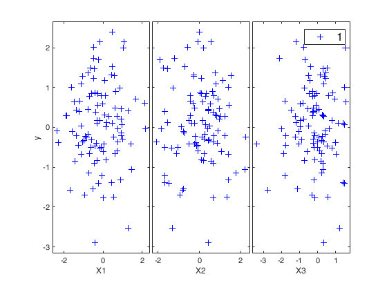
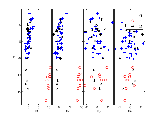
If plots = true, the yXplot that shows the response against all the explanatory variables s shown on the screen. The default value for plots is false, that is no plot is shown on the screen.
Example: 'plots',false
Data Types: single | double
pMSOM
—Proportion of MSOM outliers.the default is 10% MSOM contamination.
Example: 'pMSOM',0.25
Data Types: double
pVIOM
—Proportion of VIOM outliers (non-overlapping with MSOM).the default is 10% VIOM contamination.
Example: 'pVIOM',0.25
Data Types: double
shiftMSOMe
—Mean-shift on the error terms for MSOM outliers.default value shiftMSOMe==10.
Example: 'shiftMSOMe',-3
Data Types: double
predxMSOM
—Predictors subject to a mean shift by MSOM.it is a p-dimensional vector indexing design matrix columns.
Default value is to contaminate only the non-zero entries of beta_true (excluding the intercept).
Example: 'predxMSOM',true(2,1)
Data Types: boolean
shiftMSOMx
—Mean-shift on the predictor terms for MSOM outliers.default value shiftMSOMx==10.
Example: 'shiftMSOMx',3
Data Types: double
inflVIOMe
—Variance-inflation for the errors subject to a VIOM.default value is inflVIOMe==10.
Example: 'inflVIOMe',5
Data Types: double
Output Arguments
out — description
Structure
Structure that contains the following fields:
| Value | Description |
|---|---|
y |
simulated response. Vector. Column vector of length n containing the response. |
X |
simulated regressors. Matrix. Matrix of size n-times-nexpl containing the values of the regressors. Optional Output (for pVIOM+pMSOM>0): |
yc |
Contaminated response vector. |
Xc |
Contaminated response vector. |
ind_clean |
Indexes for non-outlying cases. |
ind_MSOM |
Indexes for MSOM outlying cases. |
ind_VIOM |
Indexes for VIOM outlying cases. |
vareps |
Variance for the uncontaminated errors. |
References
Insolia, L., F. Chiaromonte, and M. Riani (2020a).
"A Robust Estimation Approach for Mean-Shift and Variance-Inflation Outliers".
Festschrift in Honor of R. Dennis Cook pp 17–41.
See Also

|
simdatasetreg |
simulateTS |
 |
|
|
Functions |
|
• The developers of the toolbox • The forward search group • Terms of Use • Acknowledgments

