simulateTS
simulateTS simulates a time series with trend, time varying seasonal, level shift and irregular component.
Description
simulateTS simulates a time series with trend (up to third order), seasonality (constant or of varying amplitude) with a different number of harmonics and a level shift. Moreover, it is possible to add to the series the effect of explanatory variables.
Same as above, but without homogenizing the y-scale.out
=simulateTS(T,
Name, Value)
Examples
 Simulated time series with linear trend.
 Simulated time series with linear trend.
A time series of 100 observations is simulated from a model that contains a linear trend (with slope 1 and intercept 0), no seasonal component, no explanatory variables and a signal to noise ratio equal to 1 (the default).
out=simulateTS(100,'plots',1);
None of the inputs for simulating residuals has been specified. The default value signal2noiseratio=1 will be considered.
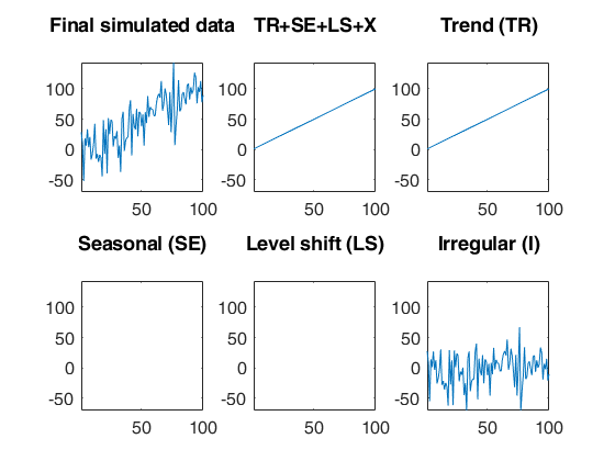
Same as above, but without homogenizing the y-scale.
close;
out=simulateTS(100,'plots',1,'samescale',false);
Related Examples
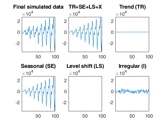
 Simulated time series with a linear time varying seasonal component.
 Simulated time series with a linear time varying seasonal component.
A time series of 100 observations is simulated from a model that contains no trend, a linear time varying seasonal component with three harmonics, no explanatory variables and a signal to noise ratio equal to 20.
rng('default')
rng(1)
model=struct;
model.trend=[];
model.trendb=[];
model.seasonal=103;
model.seasonalb=40*[0.1 -0.5 0.2 -0.3 0.3 -0.1 0.222];
model.signal2noiseratio=20;
T=100;
out=simulateTS(T,'model',model,'plots',1);
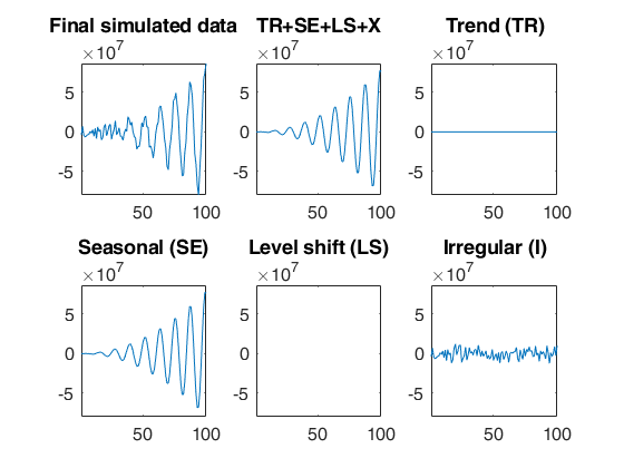
 Simulated time series with a quadratic time varying seasonal component.
 Simulated time series with a quadratic time varying seasonal component.
A time series of 100 observations is simulated from a model that contains no trend, a quadratic time varying seasonal component with one harmonic, no explanatory variables and a signal to noise ratio equal to 20.
rng(1)
model=struct;
model.trend=[];
model.trendb=[];
model.seasonal=201;
model.seasonalb=40*[0.1 -0.5 10.222 -10];
model.signal2noiseratio=20;
T=100;
out=simulateTS(T,'model',model,'plots',1);
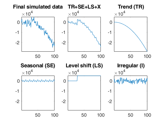
 Simulated time series with quadratic trend, fixed seasonal and level shift.
 Simulated time series with quadratic trend, fixed seasonal and level shift.
A time series of 100 observations is simulated from a model that contains a quadratic trend, a seasonal component with two harmonics, no explanatory variables and a level shift in position 30 with size 5000 and a signal to noise ratio equal to 20.
rng(1)
model=struct;
model.trend=2;
model.trendb=[5,10,-3];
model.seasonal=2;
model.seasonalb=100*[2 4 0.1 8];
model.signal2noiseratio=20;
model.lshift=30;
model.lshiftb=5000;
T=100;
out=simulateTS(T,'model',model,'plots',1);
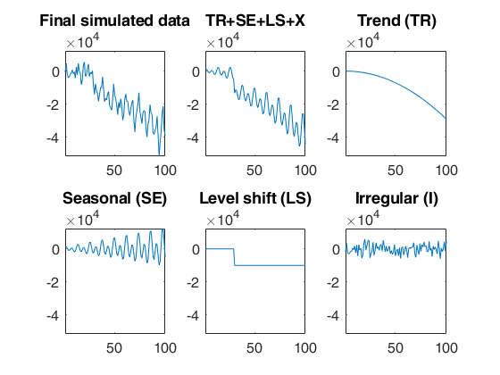
 Simulated time series with quadratic trend, fixed seasonal and LS.
 Simulated time series with quadratic trend, fixed seasonal and LS.
A time series of 100 observations is simulated from a model that contains a quadratic trend, a linear time varying seasonal component with two harmonics, no explanatory variables and a level shift in position 30 with size -10000 and a signal to noise ratio equal to 20.
rng(1)
model=struct;
model.trend=2;
model.trendb=[5,10,-3];
model.seasonal=102;
model.seasonalb=100*[2 4 0.1 8 0.001];
model.signal2noiseratio=20;
model.lshift=30;
model.lshiftb=-10000;
T=100;
out=simulateTS(T,'model',model,'plots',1);
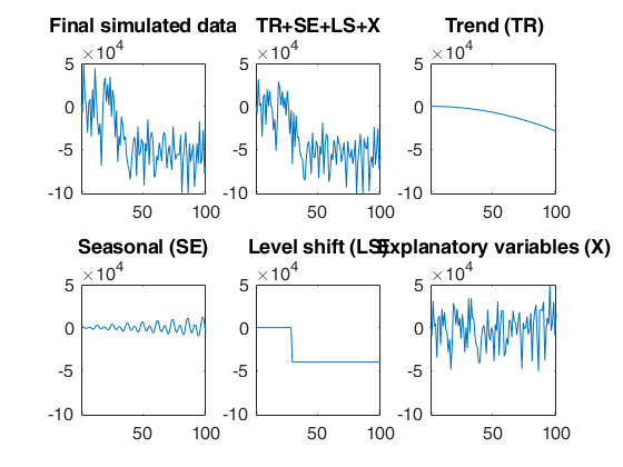
 Simulated time series with quadratic trend, fixed seasonal, LS and two explanatory variables.
 Simulated time series with quadratic trend, fixed seasonal, LS and two explanatory variables.
A time series of 100 observations is simulated from a model that contains a quadratic trend, a linear time varying seasonal component with two harmonics, two explanatory variables and a level shift in position 30 with size -40000 and a signal to noise ratio equal to 10.
rng(1)
model=struct;
model.trend=2;
model.trendb=[5,10,-3];
model.seasonal=102;
model.seasonalb=100*[2 4 0.1 8 0.001];
model.signal2noiseratio=10;
model.lshift=30;
model.lshiftb=-40000;
model.X=2;
model.Xb=[10000 20000];
T=100;
out=simulateTS(T,'model',model,'plots',1);
Example of the use of option FileNameOutput.
In this example, the simulated time series is saved into a file named ysimout.txt in the current folder.
FileNameOutput=[pwd filesep 'ysimout.txt'];
T=100;
out=simulateTS(T,'FileNameOutput',FileNameOutput);
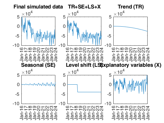
 Example of the use of option StartDate.
 Example of the use of option StartDate.
Suppose that the initial observation refers to February 2016.
StartDate=[2016 2];
% The x axis of the plots contains the dates using format mmm-yy.
rng(1)
model=struct;
model.trend=2;
model.trendb=[5,10,-3];
model.seasonal=102;
model.seasonalb=100*[2 4 0.1 8 0.001];
model.signal2noiseratio=10;
model.lshift=30;
model.lshiftb=-40000;
model.X=2;
model.Xb=[10000 20000];
T=100;
out=simulateTS(T,'model',model,'plots',1,'StartDate',StartDate);
Example of the use of option samescale.
Use a different scale for each panel in the output plot.
rng(1)
model=struct;
model.trend=2;
model.trendb=[5,10,-3];
model.seasonal=102;
model.seasonalb=100*[2 4 0.1 8 0.001];
model.signal2noiseratio=10;
model.lshift=30;
model.lshiftb=-40000;
model.X=2;
model.Xb=[10000 20000];
T=100;
out=simulateTS(T,'model',model,'plots',1,'samescale',false);
Simulated data with linear trend and errors with AR(2) component.
No seasonal component.
rng('default')
rng(100)
model=struct;
model.trend=1;
model.trendb=[5,1000];
model.seasonal='';
model.signal2noiseratio=10;
model.ARp=[1 2];
model.ARb=[0.2 0.7];
T=100;
out=simulateTS(T,'model',model,'plots',1);
y=out.y;
% The lines below just work if the econometric toolbox is present.
% The autocorrelation function of y shows just two peaks in
% correspondence of the first two lags.
if exist('parcorr','file')>0
figure
parcorr(out.y)
end
Example of simulation and fitting.
Simulated data with linear trend, errors with AR(2) component and 1 explanatory variable.
rng(100)
model=struct;
model.trend=1;
model.trendb=[5,1000];
model.seasonal='';
model.signal2noiseratio=10;
model.ARp=[1 2];
model.ARb=[0.2 0.7];
T=100;
X=1e+2*randn(T,1);
model.X=X;
model.Xb=100;
out=simulateTS(T,'model',model,'plots',1);
y=out.y;
% Fit a model with linear trend, AR(3) and the true expl. variable
model=struct;
model.trend=1;
model.seasonal=0;
model.lshift=0;
model.X=X;
model.ARp=[1 2 3];
out=LTSts(y,'model',model,'plots',1,'dispresults',true);
Input Arguments
T — time series length.
Scalar.
T is a positive integer which defines the length of the simulated time series.
Data Types: single| double
Name-Value Pair Arguments
Specify optional comma-separated pairs of Name,Value arguments.
Name is the argument name and Value
is the corresponding value. Name must appear
inside single quotes (' ').
You can specify several name and value pair arguments in any order as
Name1,Value1,...,NameN,ValueN.
 'model', model
, 'plots',1
, 'StartDate',[2016,3]
, 'nocheck',false
, 'FileNameOutput',['C:' filesep 'myoutput' filesep 'savesimdata.txt']
, 'samescale',false
model
—model type.structure.
A structure that specifies the model used to simulate the time series. The structure contains the following fields:
| Value | Description |
|---|---|
trend |
scalar (order of the trend component). trend = 1 implies linear trend with intercept, trend = 2 implies quadratic trend, etc. If this field is empty, the simulated time series will not contain a trend. The default value of model.trend is 1. |
trendb |
vector of doubles containing the beta coefficients for the trend. For example, model.trend=1 and model.trendb=[3.2 2] generate a linear trend of the kind 3.2+2*t. If this field is an empty double, the simulated time series will not contain a trend. The default value of model.trendb is [0 1], that is a slope equal to 1 and intercept equal to 0. |
s |
scalar greater than zero which specifies the length of the seasonal period. For monthly data (default) s=12, for quarterly data s=4, ... The default value of model.s is 12, which is for monthly data. |
seasonal |
scalar. Integer specifying the number of frequencies, i.e. harmonics, in the seasonal component. Possible values are , where [s/2]=floor(s/2). For example: if seasonal = 1 (default) we have: \beta_1 \cos( 2 \pi t/s) + \beta_2 \sin (2 \pi t/s); if seasonal = 2 we have: \beta_1 \cos( 2 \pi t/s) + \beta_2 \sin (2 \pi t/s) + \beta_3 \cos(4 \pi t/s) + \beta_4 \sin (4 \pi t/s). Note that when s is even, the sine term disappears for j=s/2 and so the maximum number of trigonometric parameters is s-1. If seasonal is a number greater than 100, then it is possible to specify how the seasonal component grows over time. For example, seasonal = 101 implies a seasonal component that just uses one frequency, which grows linearly over time as follows: (1+\beta_3 t)\times ( \beta_1 cos( 2 \pi t/s) + \beta_2 \sin ( 2 \pi t/s)). For example, seasonal = 201 implies a seasonal component that just uses one frequency, which grows in a quadratic way over time as follows: (1+\beta_3 t + \beta_4 t^2)\times( \beta_1 \cos( 2 \pi t/s) + \beta_2 \sin ( 2 \pi t/s)). If this field is an empty double (default), the simulated time series will not contain a seasonal component. |
seasonalb |
vector of doubles containing the beta coefficients for the seasonal component. For example, model.seasonal = 201 and model model.trendb = [1.2 2.3 3.4 4.5] generates a seasonal component of the kind: (1+ 3.4 t + 4.5 t^2)\times( 1.2 \cos( 2 \pi t/s) + 2.3 \sin ( 2 \pi t/s)). If this field is an empty double (default), the simulated time series will not contain a seasonal component. |
X |
scalar or matrix of size T-by-nexpl. If model.X is a matrix of size T-by-nexpl, it contains the values of nexpl extra covariates that affect y. If model.X is a scalar equal to k, where k=1, 2, ... k explanatory variables using random numbers from the normal distribution are generated. If this field is an empty double (default), the simulated time series will not contain explanatory variables. |
Xb |
vector of doubles containing the beta coefficients for the explanatory variables. For example, model.X = 2 and model.Xb = [4,5] generate two additional explanatory variables of the kind: 4*randn(T,1) + 5*randn(T,1) . If this field is an empty double (default), the simulated time series will not contain explanatory variables. |
ARIMAX |
boolean variable (true/false) that specifies the model for the AR component (when present). If true, then the autoregressive component involves the dependent variable, as in expression (1) of https://it.mathworks.com/help/econ/convert-between-armax-and-regarima-models.html#btw30mu with N(L)=1. If false, then the autoregressive component involves the residual term, as in expression (2) of the same page with A(L)=1. If this field is empty or not present, the default value is false. |
ARp |
vector with non-negative integer numbers specifying the autoregressive components. For example: model.ARp=[1 2] means a AR(2) process; model.ARp=2 means just the lag 2 component; model.ARp=[1 2 5 8] means AR(2) + lag 5 + lag 8; model.ARp=0 (default) means no autoregressive component. |
ARb |
vector of doubles containing the beta coefficients for the autoregressive component. For example model.ARb = [0.5 -0.2] in combination with model.ARp=[1 2] and ARIMAX=true generates an AR(2) time series of the kind: y_t = 0.5 y_{t-1} - 0.2 y_{t-2} + seasonal + lshift + \epsilon_t. model.ARb must have the same number of elements of model.ARp. If this field is an empty double (default), the simulated time series will not have an autoregressive component. |
lshift |
scalar greater than 0, which specifies the position where to include a level shift component. If this field is an empty double (default), the simulated time series will not contain a level shift. |
lshiftb |
scalar double, which specifies the magnitude of the level shift component. For example, model.lshift = 26 and model.lshiftb = 3 generates the following explanatory variable [zeros(25,1) + 3*ones(T-25+1,1)] . If this field is an empty double (default), the simulated time series will not contain a level shift. |
nsim |
scalar that defines the number of time series to simulate. If this field is empty or not present, the default value of 1 is used. |
residuals |
T x nsim matrix of doubles of length T containing the values of the residuals to use in the simulation. Default value is []. |
sigmaeps |
scalar that defines the standard error of the residuals. If model.residuals is not empty, the value of model.sigmaeps will be ignored. Default value is []. |
signal2noiseratio |
scalar that defines the ratio between the variance of the systematic part of the model (signal) and the variance of the noise (irregular model). The greater is this value, the smaller is the effect of the irregular component. If one between model.residuals and model.sigmaeps is not empty, the value of model.signal2noiseratio will be ignored. If both model.residuals and model.sigmaeps are empty and model.ARIMAX is true, then an algorithm will search the best value of the standard error of the residuals that guarantees the desired model.signal2noiseratio. If this field is empty or not present, the default value of 1 is used. Remark: the default model is for monthly data with a linear trend with slope 1 and intercept 0, no seasonal, no level shift and a signal to noise ratio equal to 1, that is: model=struct; model.s=[]; model.trend=1; model.trendb=[0 1]; model.X=[]; model.lshift=[]; model.signal2noiseratio=1; |
Example: 'model', model
Data Types: struct
plots
—Plots on the screen.scalar.
If plots == 1, a six panel plot appears on the screen.
Top left panel contains the simulated time series y.
y=TR+SE+X+LS+I of the first simulated time series.
Top central panel contains the signal component (that is, trend + seasonal + explanatory variables + level shift = TR + SE + LS + X).
Top right panel contains the trend component (TR).
Bottom left panel contains the (time varying) seasonal component (SE).
Bottom central panel contains the level shift component (LS).
Bottom right panel contains the explanatory variable component (X) if it is present, otherwise, it contains the irregular (I) component of the first simulation.
The default value of plot is 0, that is no plot is shown on the screen.
Example: 'plots',1
Data Types: double
StartDate
—The time of the first observation.numeric vector of length 2.
Vector with two integers, which specify a natural time unit and a (1-based) number of samples into the time unit. For example, if model.s=12 (that is the data are monthly) and the first observation starts in March 2016, then StartDate=[2016,3]; similarly, if models.s=4 (that is the data are quarterly) and the first observation starts in the second quarter or year 2014, then StartData=[2014,2]. The information in option StartDate will be used to create in the output the dates inside the time series object.
Example: 'StartDate',[2016,3]
Data Types: double
nocheck
—Check input arguments.boolean.
If nocheck is true, no check is performed on supplied input. Otherwise (default), every input of the structure model is checked.
Example: 'nocheck',false
Data Types: double
FileNameOutput
—save simulated time series to txt file.character.
If FileNameOutput is empty (default), nothing is saved on the disk, else FileNameOutput will contain the path where to save the file on the disk.
Example: 'FileNameOutput',['C:' filesep 'myoutput' filesep 'savesimdata.txt']
Data Types: Character
samescale
—same ylim in the output plot.logical.
If true (default), all underlying components of the time series are shown in the plot with the same scale.
Example: 'samescale',false
Data Types: logical
Output Arguments
out — description
Structure
Structure that contains the following fields:
| Value | Description |
|---|---|
y |
the simulated time series. Matrix of dimension T x nsim, which is sum of trend + (time varying) seasonal + explanatory variables + level shift + irregular = TR+SE+X+LS+I. |
signal |
signal (TR+SE+X+LS). Column vector of length T, which is sum of trend + (time varying) seasonal + explanatory variables + level shift. Signal = out.y - out.irregular. |
trend |
trend (TR). Column vector of length T, which contains the trend component. |
seasonal |
(time varying) seasonal (SE). Column vector of length T, which contains the seasonal component. If there is no seasonal component: outyhatseaso=0. |
X |
explanatory variables (X). Column vector of length T, which contains the component associated to the explanatory variables. If there is no explanatory variable, out.X=0. |
lshift |
level shift (LS). Column vector of length T, which contains the level shift component. If there is no level shift component out.lshift=0. |
irregular |
irregular component (I). Matrix of dimension T x nsim, which contains the irregular component. When the signal to noise ratio tends to infinity, the irregular component tends to 0. |
model |
structure. The model used to simulate the time series. |
References
Rousseeuw, P.J., Perrotta D., Riani M. and Hubert, M. (2018), Robust Monitoring of Many Time Series with Application to Fraud Detection, "Econometrics and Statistics". [RPRH]