simulateLM
simulateLM simulates linear regression data with pre-specified values of statistical indexes.
Description
simulateLM simulates linear regression data. It is possible to specify:
1) the requested value of R2 (or equivalently its SNR);
2) the values of the beta coefficients (possibly sparse);
3) the correlation (covariance) matrix among the explanatory variables.
4) the value of the intercept term.
5) the distribution to use to generate the Xs;
6) the distribution to use to generate the ys.
7) the MSOM contamination in Xs and ys.
8) the VIOM contamination in ys.
Simulate with prefixed value of R2.out
=simulateLM(n,
Name, Value)
Examples
 Use all default options.
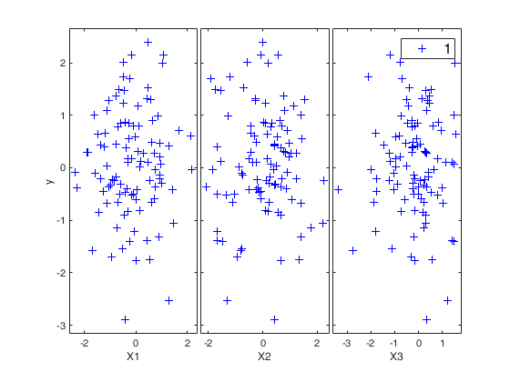
Use all default options.Simulate 100 observations y and X (uncorrelated with y) using standard normal distribution.
out=simulateLM(100,'plots',true);
Simulate with prefixed value of R2.
Simulate with prefixed value of R2.Set value of R2;
R2=0.82;
n=10000;
out=simulateLM(n,'R2',R2);
outLM=fitlm(out.X,out.y);
Related Examples
Use prefixed correlation matrix for cov(X).
Use prefixed correlation matrix for cov(X).Set value of R2;
R2=0.26;
n=10000;
A = gallery('moler',5,0.2);
out=simulateLM(n,'R2',R2,'SigmaX',A);
outLM=fitlm(out.X,out.y)
outLM =


Linear regression model:
    y ~ 1 + x1 + x2 + x3 + x4 + x5

Estimated Coefficients:
                   Estimate        SE        tStat       pValue
                   _________    ________    _______    __________

    (Intercept)    -0.076653    0.053898    -1.4222       0.15501
    x1                1.0515    0.056414     18.638    3.0647e-76
    x2               0.92447    0.056001     16.508    2.0145e-60
    x3                1.0394    0.055297     18.797      1.72e-77
    x4               0.92012    0.055248     16.654    1.8903e-61
    x5                 1.029    0.054653     18.828    9.8022e-78


Number of observations: 10000, Error degrees of freedom: 9994
Root Mean Squared Error: 5.39
R-squared: 0.253,  Adjusted R-Squared: 0.253
F-statistic vs. constant model: 679, p-value = 0
Use prefixed values of R2, beta and intercept.
Use prefixed values of R2, beta and intercept.Set value of R2.
R2=0.92;
beta=[3; 4; 5; 2; 7];
intercept=true;
n=100000;
out=simulateLM(n,'R2',R2,'beta',beta);
outLM=fitlm(out.X,out.y);
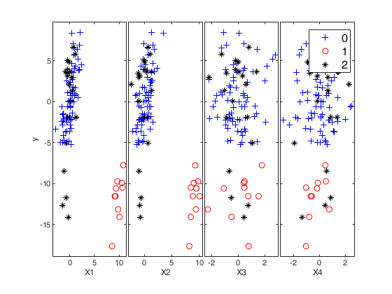
Use SNR and include MSOM (on active features) and VIOM contamination.
Use SNR and include MSOM (on active features) and VIOM contamination.%% Use SNR and include MSOM (on active features) and VIOM contamination. SNR=3; beta=[2, 2, 0, 0]; intercept=true; n=100; out=simulateLM(n,'SNR',SNR,'beta',beta, 'pMSOM', 0.1, 'pVIOM', 0.2, 'plots', 1); X = out.X; y = out.y; outLM=fitlm(X,y); Xc = out.Xc; yc = out.yc; outLM2=fitlm(Xc,yc);
Input Arguments
Output Arguments
References
Insolia, L., F. Chiaromonte, and M. Riani (2020a).
"A Robust Estimation Approach for Mean-Shift and Variance-Inflation Outliers".
Festschrift in Honor of R. Dennis Cook pp 17–41.