FSReda

FSReda enables to monitor several quantities in each step of the forward search

Syntax

Description

example

out =FSReda(y, X, bsb) FSReda with all default options.

example

out =FSReda(y, X, bsb, Name, Value) FSReda with optional argument.

Examples

expand all

  • FSReda with all default options.
  • Example of use of FSReda based on a starting point coming from LMS.

    n=200;
    p=3;
    randn('state', 123456);
    X=randn(n,p);
    % Uncontaminated data
    y=randn(n,1);
    % Contaminated data
    ycont=y;
    ycont(1:5)=ycont(1:5)+6;
    [out]=LXS(y,X,'nsamp',1000);
    out=FSReda(y,X,out.bs);

  • FSReda with optional argument.
  • Example of use of function FSReda using a random start and traditional t-stat monitoring.

    n=200;
    p=3;
    randn('state', 123456);
    X=randn(n,p);
    % Uncontaminated data
    y=randn(n,1);
    % Contaminated data
    ycont=y;
    ycont(1:5)=ycont(1:5)+6;
    out=FSReda(y,X,0,'tstat','trad');

    Related Examples

    expand all

  • Examples with real data: wool data.
  • xx=load('wool.txt');
    X=xx(:,1:3);
    y=log(xx(:,4));
    [out]=LXS(y,X,'nsamp',0);
    [out]=FSReda(y,X,out.bs,'tstat','scal');

  • Example with artificial dataset.
  • n=100;
    p=8;
    state=1;
    randn('state', state);
    X=randn(n,p);
    y=randn(n,1);
    y(1:10)=y(1:10)+5;
    % Run the forward search with Exploratory Data Analysis purposes
    % LMS using 10000 subsamples
    [outLXS]=LXS(y,X,'nsamp',10000);
    % Forward Search
    [out]=FSReda(y,X,outLXS.bs);
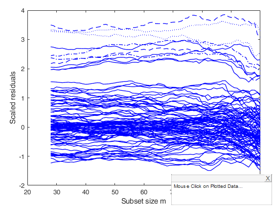
    %The monitoring residuals plot shows a set of positive residuals which
    %starting from the central part of the search tend to have a residual much
    %larger than that of the other units.
    resfwdplot(out);
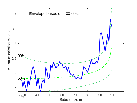
    %The minimum deletion residual from m=90 starts going above the 99% threshold.
    mdrplot(out);
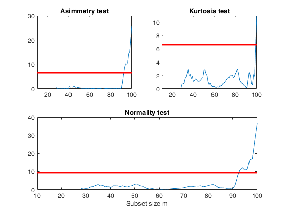
    %The curve which monitors the normality test shows a sudden big increase with the outliers are included
    figure;
    lwdenv=2;
    xlimx=[10 100];
    subplot(2,2,1);
    plot(out.nor(:,1),out.nor(:,2));
    title('Asimmetry test');
    xlim(xlimx);
    quant=chi2inv(0.99,1);
    v=axis;
    line([v(1),v(2)],[quant,quant],'color','r','LineWidth',lwdenv);
    subplot(2,2,2)
    plot(out.nor(:,1),out.nor(:,3))
    title('Kurtosis test');
    xlim(xlimx);
    v=axis;
    line([v(1),v(2)],[quant,quant],'color','r','LineWidth',lwdenv);
    subplot(2,2,3:4)
    plot(out.nor(:,1),out.nor(:,4));
    xlim(xlimx);
    quant=chi2inv(0.99,2);
    v=axis;
    line([v(1),v(2)],[quant,quant],'color','r','LineWidth',lwdenv);
    title('Normality test');
    xlabel('Subset size m');
    Total estimated time to complete LMS:  0.04 seconds 
    
    Click here for the graphical output of this example (link to Ro.S.A. website)

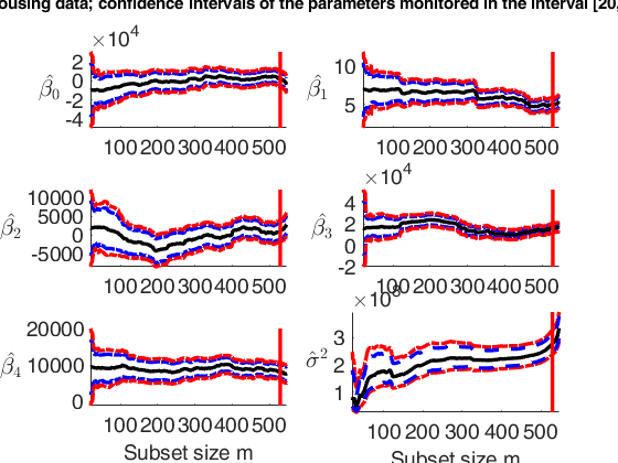
  • Monitoring of 95 per cent and 99 per cent confidence intervals of beta and sigma2.
  • % House price data
    load hprice.txt;
    n=size(hprice,1);
    y=hprice(:,1);
    X=hprice(:,2:5);
    outFSR=FSR(y,X,'plots',0,'msg',0);
    dout=n-length(outFSR.ListOut);
    % init = point to start monitoring diagnostics along the FS
    init=20;
    [outLXS]=LXS(y,X,'nsamp',10000);
    outEDA=FSReda(y,X,outLXS.bs,'conflev',[0.95 0.99],'init',init);
    p=size(X,2)+1;
    % Set font size, line width and line style
    figure;
    lwd=2.5;
    FontSize=14;
    linst={'-','--',':','-.','--',':'};
    nr=3;
    nc=2;
    xlimL=init; % lower value fo xlim
    xlimU=n+1;  % upper value of xlim
    close all
    for j=1:p
    subplot(nr,nc,j);
    hold('on')
    % plot 95% and 99% HPD  trajectories
    plot(outEDA.Bols(:,1),outEDA.betaINT(:,1:2,j),'LineStyle',linst{4},'LineWidth',lwd,'Color','b')
    plot(outEDA.Bols(:,1),outEDA.betaINT(:,3:4,j),'LineStyle',linst{4},'LineWidth',lwd,'Color','r')
    % plot estimate of beta1_j
    plot(outEDA.Bols(:,1),outEDA.Bols(:,j+1)','LineStyle',linst{1},'LineWidth',lwd,'Color','k')
    % Set ylim
    ylimU=max(outEDA.betaINT(:,4,j));
    ylimL=min(outEDA.betaINT(:,3,j));
    ylim([ylimL ylimU])
    % Set xlim
    xlim([xlimL xlimU]);
    % Add vertical line in correspondence of the step prior to the
    % entry of the first outlier
    line([dout; dout],[ylimL; ylimU],'Color','r','LineWidth',lwd);
    ylabel(['$\hat{\beta_' num2str(j-1) '}$'],'Interpreter','LaTeX','FontSize',20,'rot',-360);
    set(gca,'FontSize',FontSize);
    if j>(nr-1)*nc
    xlabel('Subset size m','FontSize',FontSize);
    end
    end
    % Subplot associated with the monitoring of sigma^2
    subplot(nr,nc,6);
    hold('on')
    % 99%
    plot(outEDA.sigma2INT(:,1),outEDA.sigma2INT(:,4:5),'LineStyle',linst{4},'LineWidth',lwd,'Color','r')
    % 95%
    plot(outEDA.sigma2INT(:,1),outEDA.sigma2INT(:,2:3),'LineStyle',linst{2},'LineWidth',lwd,'Color','b')
    % Plot rescaled S2
    plot(outEDA.S2(:,1),outEDA.S2(:,4),'LineWidth',lwd,'Color','k')
    ylabel('$\hat{\sigma}^2$','Interpreter','LaTeX','FontSize',20,'rot',-360);
    set(gca,'FontSize',FontSize);
    % Set ylim
    ylimU=max(outEDA.sigma2INT(:,5));
    ylimL=min(outEDA.sigma2INT(:,4));
    ylim([ylimL ylimU])
    % Set xlim
    xlim([xlimL xlimU]);
    % Add vertical line in correspondence of the step prior to the
    % entry of the first outlier
    line([dout; dout],[ylimL; ylimU],'Color','r','LineWidth',lwd);
    xlabel('Subset size m','FontSize',FontSize);
    % Add multiple title
    suplabel(['Housing data; confidence intervals of the parameters monitored in the interval ['...
    num2str(xlimL) ',' num2str(xlimU) ...
    ']'],'t');
    disp(['The vertical lines are located in the' ...
    ' step prior to the inclusion of the first outlier'])
    Total estimated time to complete LMS:  0.18 seconds 
    ------------------------------
    Warning: Number of subsets without full rank equal to 38.3%
    m=100
    m=200
    m=300
    m=400
    m=500
    The vertical lines are located in the step prior to the inclusion of the first outlier
    
    Click here for the graphical output of this example (link to Ro.S.A. website)

  • Interactive example 1. Reveal masked outliers.
  • % Load the data
    clearvars;close all;
    load('multiple_regression.txt');
    y=multiple_regression(:,4);
    X=multiple_regression(:,1:3);
    % yX plot
    yXplot(y,X)
    % Robust analysis
    % LMS using 1000 subsamples
    [out]=LXS(y,X,'nsamp',10000);
    % Forward Search
    [out]=FSReda(y,X,out.bs);
    out1=out;
    % Create scaled squared residuals
    out1.RES=out.RES.^2;
    resfwdplot(out1,'databrush',1);

  • Example to compute REML single weights for the units excluded from the search at each step using wREML=true.
  • load('loyalty.mat');
    y = loyalty{:,end};
    X = loyalty{:,1};
    tit = sprintf('Loyalty data');
    xla = 'Number of visits';
    yla = 'Amount spent (in Euros)';
    n = size(X, 1);
    p = size(X, 2);
    % LXS and FSReda
    [outLXS]=LXS(y,X,'nsamp',1000);
    [out] = FSReda(y, X, outLXS.bs, 'intercept', false, 'wREML', true);
    % plot solution overwriting the RES output for simplicity
    out.RES = out.wREML;
    resfwdplot(out);
    ylabel('REML weights FS');
    Total estimated time to complete LMS:  0.01 seconds 
    m=100
    m=200
    m=300
    m=400
    m=500
    
    Click here for the graphical output of this example (link to Ro.S.A. website)

    Input Arguments

    expand all

    y — Response variable. Vector.

    Response variable, specified as a vector of length n, where n is the number of observations. Each entry in y is the response for the corresponding row of X.

    Missing values (NaN's) and infinite values (Inf's) are allowed, since observations (rows) with missing or infinite values will automatically be excluded from the computations.

    Data Types: single| double

    X — Data matrix of explanatory variables (also called 'regressors') of dimension (n x p-1). Rows of X represent observations, and columns represent variables.

    Missing values (NaN's) and infinite values (Inf's) are allowed, since observations (rows) with missing or infinite values will automatically be excluded from the computations.

    Data Types: single| double

    bsb — list of units forming the initial subset. Vector or scalar.

    If bsb=0 (default) then the procedure starts with p units randomly chosen else if bsb is not 0 the search will start with m0=length(bsb).

    Data Types: single| double

    Name-Value Pair Arguments

    Specify optional comma-separated pairs of Name,Value arguments. Name is the argument name and Value is the corresponding value. Name must appear inside single quotes (' '). You can specify several name and value pair arguments in any order as Name1,Value1,...,NameN,ValueN.

    Example: 'conflev',[0.90 0.93] , 'init',100 starts monitoring from step m=100 , 'intercept',false , 'nocheck',true , 'tstat','trad' , 'wREML', true

    conflev —confidence levels to be used to compute confidence interval for the elements of $\beta$ and for $\sigma^2$.vector.

    The default value of conflev is [0.95 0.99] that is 95% and 99% confidence intervals are computed.

    Example: 'conflev',[0.90 0.93]

    Data Types: double

    init —Search initialization.scalar.

    It specifies the point where to initialize the search and start monitoring required diagnostics. if init is not specified it will be set equal to : p+1, if the sample size is smaller than 40;

    min(3*p+1,floor(0.5*(n+p+1))), otherwise.

    Example: 'init',100 starts monitoring from step m=100

    Data Types: double

    intercept —Indicator for constant term.true (default) | false.

    Indicator for the constant term (intercept) in the fit, specified as the comma-separated pair consisting of 'Intercept' and either true to include or false to remove the constant term from the model.

    Example: 'intercept',false

    Data Types: boolean

    nocheck —Check input arguments.boolean.

    If nocheck is equal to true no check is performed on matrix y and matrix X. Notice that y and X are left unchanged. In other words the additional column of ones for the intercept is not added. As default nocheck=false. The controls on h, alpha and nsamp still remain

    Example: 'nocheck',true

    Data Types: boolean

    tstat —the kind of t-statistics which have to be monitored.character.

    tstat = 'trad' implies monitoring of traditional t statistics (out.Tols). In this case the estimate of $\sigma^2$ at step m is based on $s^2_m$ (notice that $s^2_m<<\sigma^2$ when m/n is small) tstat = 'scal' (default) implies monitoring of rescaled t statistics In this case the estimate of $\sigma^2$ at step m is based on $s^2_m / var_{truncnorm(m/n)}$ where $var_{truncnorm(m/n)}$ is the variance of the truncated normal distribution.

    Example: 'tstat','trad'

    Data Types: char

    wREML —compute REML weights for unit excluded from FS at each step.false (default) | true.

    If weak==true REML weights are computed.

    Example: 'wREML', true

    Data Types: boolean Data Types - double

    Output Arguments

    expand all

    out — description Structure

    Structure which contains the following fields

    Value Description
    RES

    n x (n-init+1) = matrix containing the monitoring of scaled residuals: 1st row = residual for first unit;

    ...;

    nth row = residual for nth unit.

    LEV

    (n+1) x (n-init+1) = matrix containing the monitoring of leverage: 1st row = leverage for first unit: ...;

    nth row = leverage for nth unit.

    BB

    n x (n-init+1) matrix containing the information about the units belonging to the subset at each step of the forward search: 1st col = indexes of the units forming subset in the initial step;

    ...;

    last column = units forming subset in the final step (all units).

    mdr

    n-init x 3 matrix which contains the monitoring of minimum deletion residual or (m+1)ordered residual at each step of the forward search: 1st col = fwd search index (from init to n-1);

    2nd col = minimum deletion residual;

    3rd col = (m+1)-ordered residual.

    Remark: these quantities are stored with sign, that is the min deletion residual is stored with negative sign if it corresponds to a negative residual.

    msr

    n-init+1 x 3 = matrix which contains the monitoring of maximum studentized residual or m-th ordered residual: 1st col = fwd search index (from init to n);

    2nd col = maximum studentized residual;

    3rd col = (m)-ordered studentized residual.

    nor

    (n-init+1) x 4 matrix containing the monitoring of normality test in each step of the forward search: 1st col = fwd search index (from init to n);

    2nd col = Asymmetry test;

    3rd col = Kurtosis test;

    4th col = Normality test.

    Bols

    (n-init+1) x (p+1) matrix containing the monitoring of estimated beta coefficients in each step of the forward search.

    S2

    (n-init+1) x 5 matrix containing the monitoring of S2 or R2, F test, in each step of the forward search: 1st col = fwd search index (from init to n);

    2nd col = monitoring of S2;

    3rd col = monitoring of R2;

    4th col = monitoring of rescaled S2.

    In this case the estimated of $\sigma^2$ at step m is divided by the consistency factor (to make the estimate asymptotically unbiased).

    5th col = monitoring of F test. Note that an asymptotic unbiased estimate of sigma2 is used.

    coo

    (n-init+1) x 3 matrix containing the monitoring of Cook or modified Cook distance in each step of the forward search: 1st col = fwd search index (from init to n);

    2nd col = monitoring of Cook distance;

    3rd col = monitoring of modified Cook distance.

    Tols

    (n-init+1) x (p+1) matrix containing the monitoring of estimated t-statistics (as specified in option input 'tstat'.

    in each step of the forward search

    Un

    (n-init) x 11 Matrix which contains the unit(s) included in the subset at each step of the fwd search.

    REMARK: in every step the new subset is compared with the old subset. Un contains the unit(s) present in the new subset but not in the old one Un(1,2) for example contains the unit included in step init+1 Un(end,2) contains the units included in the final step of the search.

    betaINT

    Confidence intervals for the elements of $\beta$.

    betaINT is a (n-init+1)-by-2*length(confint)-by-p 3D array.

    Each third dimension refers to an element of beta: betaINT(:,:,1) is associated with first element of beta;

    ...;

    betaINT(:,:,p) is associated with last element of beta.

    The first two columns contain the lower and upper confidence limits associated with conflev(1).

    Columns three and four contain the lower and upper confidence limits associated with conflev(2);

    ...;

    The last two columns contain the lower and upper confidence limits associated with conflev(end).

    For example betaint(:,3:4,5) contain the lower and upper confidence limits for the fifth element of beta using confidence level specified in the second element of input option conflev.

    sigma2INT

    confidence interval for $\sigma^2$.

    1st col = fwd search index;

    2nd col = lower confidence limit based on conflev(1);

    3rd col = upper confidence limit based on conflev(1);

    4th col = lower confidence limit based on conflev(2);

    5th col = upper confidence limit based on conflev(2);

    ...

    penultimate col = lower confidence limit based on conflev(end);

    last col = upper confidence limit based on conflev(end);

    y

    A vector with n elements that contains the response variable which has been used

    X

    Data matrix of explanatory variables which has been used (it also contains the column of ones if input option intercept was missing or equal to 1)

    class

    'FSReda'.

    wREML

    Singularly optimal REML weights for the units excluded for the search at each step.

    Present only if wREML == true.

    n x (n-init+1) = matrix containing the monitoring of singlular REML weights: 1st row = weight for first unit;

    ...;

    nth row = weight for nth unit.

    References

    Atkinson, A.C. and Riani, M. (2000), "Robust Diagnostic Regression Analysis", Springer Verlag, New York.

    See Also

    |

    This page has been automatically generated by our routine publishFS